Lab Intro
The purpose of this lab is to apply what we've learned before in a practical scenario: using the ToF sensors attached on our robot to map out a static environment. To this end, we will make use of orientation control as before to make the car rotate by certain increments at select spots to scan its surroundings and produce accurate data which we can use to map out the environment. Additionally, we can adjust the number of steps / increment degree of the robot car as well in this command for increased flexibility.
Bluetooth Communication
Again, like in the previous stunt lab, we will be using a nonblocking command that can be called from our Python side which will set a flag and effectively activate a finite state machine in our Arduino code that will run the full scanning program. As shown below, because we plan to use orientation PID control, it is very helpful to add the PID variables in the input so that we may adjust our control loop on the fly without needing to reflash.
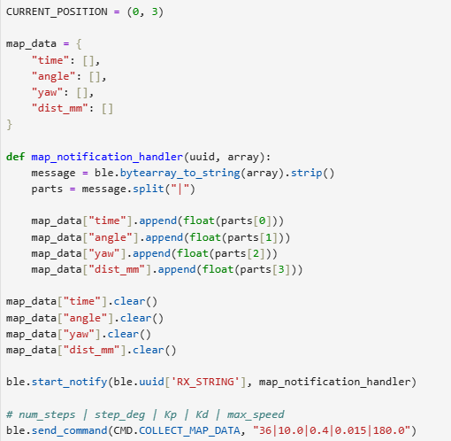 Command on Python side used to trigger the scanning.
Once received on the Arduino side, the FSM that controls the scanning will switch its state from MAP_IDLE to MAP_SETTLING, effectively telling the main loop to start looping our helper function which contains the FSM.
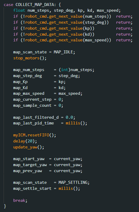 New Bluetooth command on Arduino side.
The helper function is shown below. After moving to an active state (MAP_SETTLING to start because we want to measure distance at the initial position), every time the function is looped, we will perform the run_map_scan_pid function, which is just another version of the orientation PID control that we have been using in the previous labs. This is important to ensure that the robot can reliably and accurately hit its desired yaw position and thus acquire good data. The basic flow of the FSM sees the robot car going from MAP_SETTLING to MAP_READING to MAP_TURNING and continues that cycle until we've finished a complete 360 degree scan. The purpose of the MAP_SETTLING state is to allow the robot to have enough time to stabilize before we read the ToF to ensure the data is reliable.
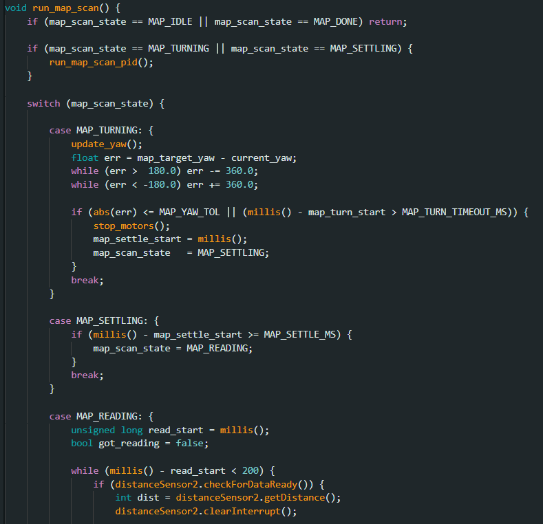 Helper function containing the mapping FSM.
Below is the PID function. It should be noted that the deadband value has been increased to 150. While making the car's rotation as a whole a bit more jittery, this was necessary as we were experiencing some issues with the wheels not turning with lower pwm values, leading the car to stray away from the scanning location.
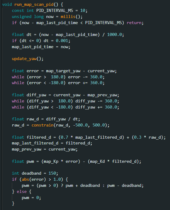 Helper function containing PID controller.
Turning Accuracy
In order to ensure that we acquired enough data to get an accurate picture of the structure, we decided to have the robot perform 36 scans for every scanning position (so increments of 10 degrees). We only used the five designated spots of (-3,-2), (5,3), (0,3), (5,-3) and (0,0) to collect our data. As seen in the plot below, the accuracy of the orientation PID was very solid, with each turn very closely matching our expected yaw value.
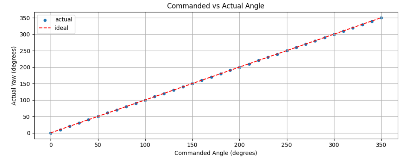 Plotting actual yaw versus ideal yaw.
Using Python, we calculated that the average angular error was 0.40 degrees, which is acceptable given increments of 10 degrees. Since a 4x4m room has walls at most 2m from the center, this angular error translates to an average positional error of 1.4 cm and maximum of 3.3 cm using the small angle approximation. The primary sources of error are DMP drift over the full 360° rotation and the robot's tendency to not turn perfectly on-axis since, as seen in the video below, the robot can be somewhat inconsistent with how much the wheels grip the surface of the floor.
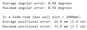 Results of our angular errors.
Video showcasing the robot turning on the spot.
Mapping Results
In order to quickly check if our data collected was reasonable or not, we plotted our data on polar plots first. In order to make our lives easier in the future for transformations, we standardized the starting angle to be 90 degrees from the positive x-axis (pointing upwards). Just by comparing what we saw in the polar plots and the actual environment, we could confirm the results were reasonable.
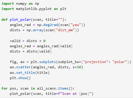 Python code used to generate the polar plots.
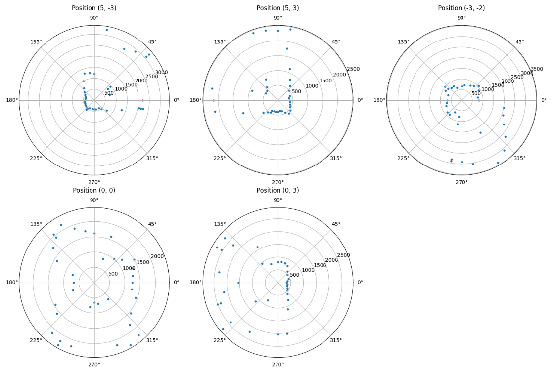 Polar plots used as a sanity check for our data.
Rather than assuming equal angular spacing between readings, we trusted the actual DMP yaw values recorded at each step, as our orientation PID controller reliably drove the robot to each target angle with low error. This ensures that any slight variation in step size is accounted for in the transformation rather than introducing systematic error by assuming uniform spacing.
Once we confirmed that the data was solid, we could then start our transformations to convert from polar coordinates to Cartesian coordinates. For each scan position, we applied a rotation matrix followed by a translation to convert each ToF reading from the robot's local frame into the global world frame. The transformation takes the form:
Transformation Matrix
| ⎡ |
xworld |
⎤ |
= |
⎡ |
cos θ |
−sin θ |
tx |
⎤ |
⎡ |
d · cos φ |
⎤ |
| ⎢ |
yworld |
⎥ |
= |
⎢ |
sin θ |
cos θ |
ty |
⎥ |
⎢ |
d · sin φ |
⎥ |
| ⎣ |
1 |
⎦ |
|
⎣ |
0 |
0 |
1 |
⎦ |
⎣ |
1 |
⎦ |
Where d is the ToF distance reading (plus the 75mm sensor offset from the center of rotation), φ is the measured yaw angle normalized to start at 0°, θ is the robot's initial heading in the world frame (90° since the robot faces the +y axis), and (tx, ty) is the known scan position in feet. Each ToF point is first expressed in the robot's local frame as a vector, then rotated by θ and translated to the world frame.
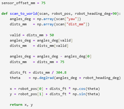 Python code used for transformation.
Now we simply plot our new set of data to see how accurately it maps the environment:
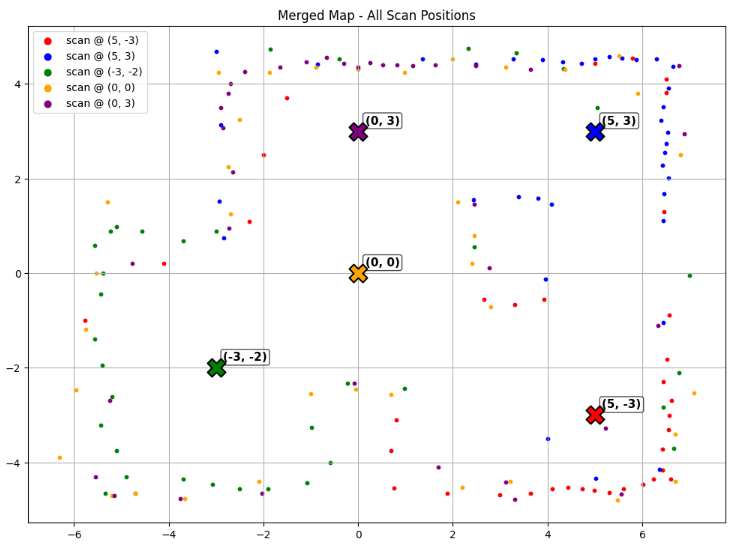 Combined map with all our data.
Fortunately, most of the data seems to line up well with one another apart from some minor discrepancies, and this allows us to pretty accurately estimate the walls of the environment as seen below. No specific points were removed, and for determining where to place the boundary lines, we chose to rely more heavily on the data collected from a closer scanning point.
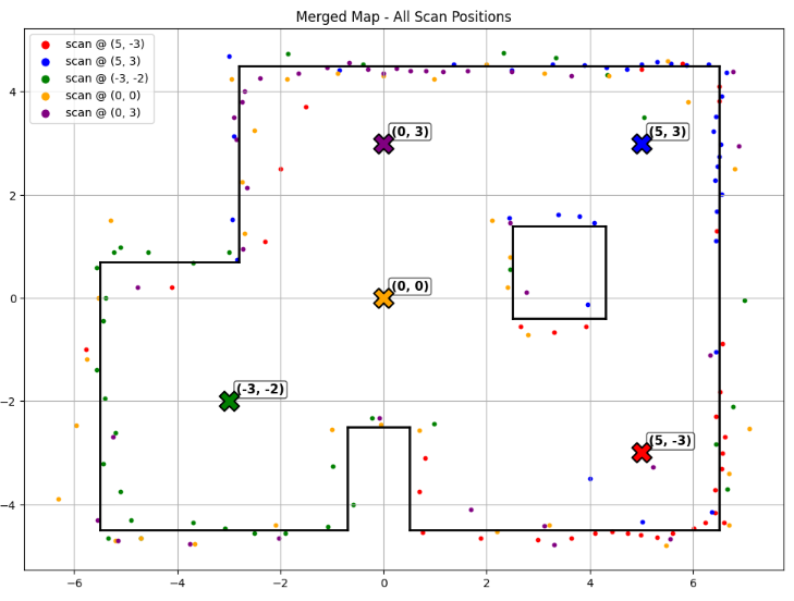 Map with lines overlaid.
As a result, the final boundaries can be described in two lists detailing the points of the lines used:
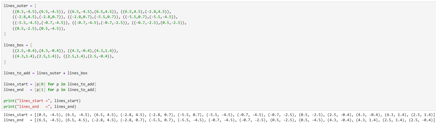 Final lists containing vertices of our boundary.
Overall, this lab was very useful in applying the concepts that we had learned before, including our orientation PID control and ToF sensors, for a practical application like environment mapping, which will directly feed into the localization and navigation tasks in future labs. Aidan McNay's website was used for inspiration on some parts of this lab.