Lab Intro
As we saw in Lab 5, the ToF sensor has limitations when in terms of sampling speed, meaning that our main control loop runs faster than the sensor can provide data and we're left with periods of time where the robot isn't acting according to the most up-to-date data, harming its ability to be responsive. One of the fixes that we've looked into was using linear extrapolation to bridge the gaps, but in this lab, we'll be exploring a much more potent solution, Kalman Filters, and their usefulness in supplementing slow ToF data.
Estimate Drag and Momentum
In order to get an in depth understanding of the system and the way it moves, we first need to estimate its drag and momentum. Using our ToF sensor and time stamped data, the strategy would be to drive the car straight into a wall at a certain known PWM value to find its steady state velocity. To this end, a Bluetooth command very similar to the ones used in previous labs was implemented to drive a continuous PWM signal until the robot reached a certain distance away from the wall.
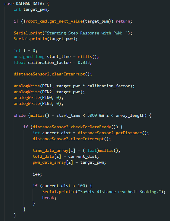 New Bluetooth command used to drive car forwards.
The lab handout suggested selecting a step response to be around 50%-100% of the maximum, or 255, so a relatively lower value of 150 was chosen, or ~59% of the max. The reasoning was that at higher speeds, the amount of data we could collect would be lower and thus less reliable for making a proper Kalman Filter. It should also be noted that the timing budget was lowered from 100 ms to 50 ms for our ToF sensor in order to collect more data points. This came at the tradeoff of affecting our maximum range, which could cause issues in preventing the car from having enough room to accelerate to steady state velocity, but due to the lower speed chosen, this wasn't a problem.
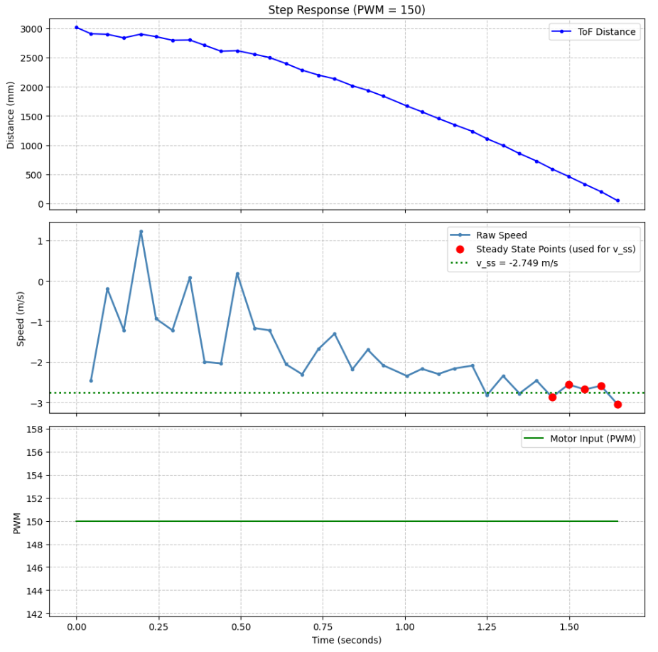
Seen below is the result of our test, and despite the relative variability in the calculated velocity of the car, it can be seen that the last five points are relatively stable, allowing us to use the mean to acquire a decent estimate for the steady state speed of around 2.749 m/s.
 Results of driving the car into a wall.
We are also asked to find the speed at 90% risetime. Since we didn't use an exponential decay function to model the velocity, we simply picked the first datapoint whose velocity crossed the 90% threshold of 2.474 m/s, which turned out to be at around 1.25 seconds.
From these two values, drag and momentum can be derived directly from first-order dynamics. At steady state, acceleration is zero, meaning the motor input exactly balances drag, giving d = u / |v_ss| where u = 150/255 is the normalized input. The time constant τ = t_90 / 2.303 follows from the first-order step response equation, and momentum is then m = d · τ.
Derived System Parameters
d = u / |vss| = (150/255) / 2.7488 = 0.2140
τ = t90 / 2.303 = 1.25 / 2.303 = 0.5428 s
m = d · τ = 0.2140 × 0.5428 = 0.1161
These parameters define the continuous time state space matrices, where the state vector is [position (mm), velocity (mm/s)]. Position integrates velocity (A[0][1] = 1), velocity decays with drag (A[1][1] = -d/m), and motor input only directly drives velocity (B[1][0] = 1/m).
Continuous Time State Space
A = [[0, 1], [0, -1.8424]]
B = [[0], [8.6096]]
Initialize KF (Python)
With A and B defined, the matrices were discretized using the average ToF sampling period of ΔT = 0.0499 s, which was measured directly from the step response data. The discretization follows Ad = I + ΔT·A and Bd = ΔT·B, converting the continuous time model into one that can be stepped forward at each sensor update.
Discretized Matrices (ΔT = 0.0499 s)
Ad = [[1.0, 0.0499], [0.0, 0.9080]]
Bd = [[0.0], [0.4297]]
The C matrix maps the state vector to what is actually measured. Since the ToF sensor returns positive distance directly, C = [1, 0], and the initial state vector was set to the first ToF reading with velocity assumed zero. Three covariance parameters were chosen to initialize the filter: σ₁ = 20mm (position process noise), σ₂ = 158 mm/s (velocity process noise), and σ₃ = 5mm (sensor noise). Their derivation and tuning is discussed in the next section.
Python KF Sanity Check
Before implementing on the Artemis, the Kalman Filter was tested in Jupyter using the step response data collected earlier. Since the KALMAN_DATA command logs one PWM value per ToF reading, the arrays were already equal length and no extrapolation was needed. The KF function follows the standard predict-update cycle: the predict step propagates the state forward using the discretized model, and the update step corrects the prediction using the new ToF measurement weighted by the Kalman gain.
The input was normalized by dividing by the step size of 150 to match the scale used when deriving the B matrix. The filter was initialized with the first ToF reading as position and zero velocity. Shown below is the resulting KF estimate plotted against the raw ToF data.
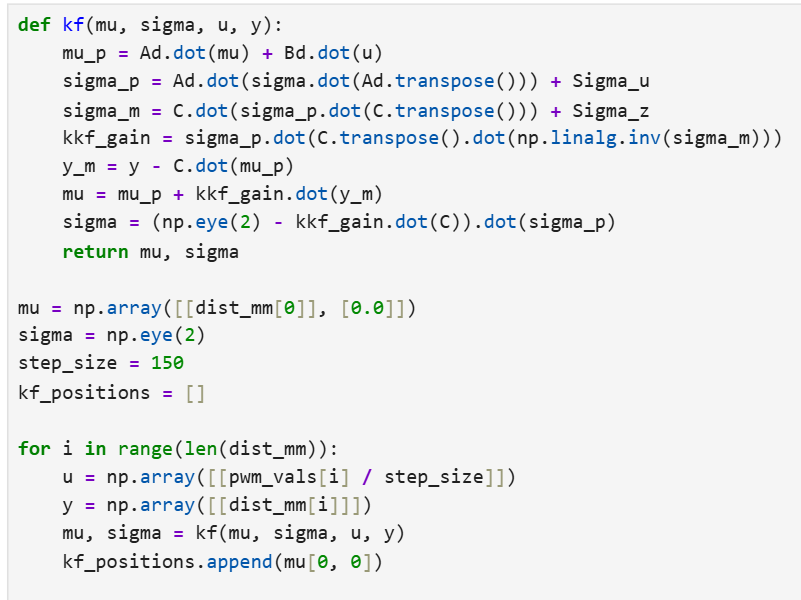 Code used to test derived Kalman Filter values.
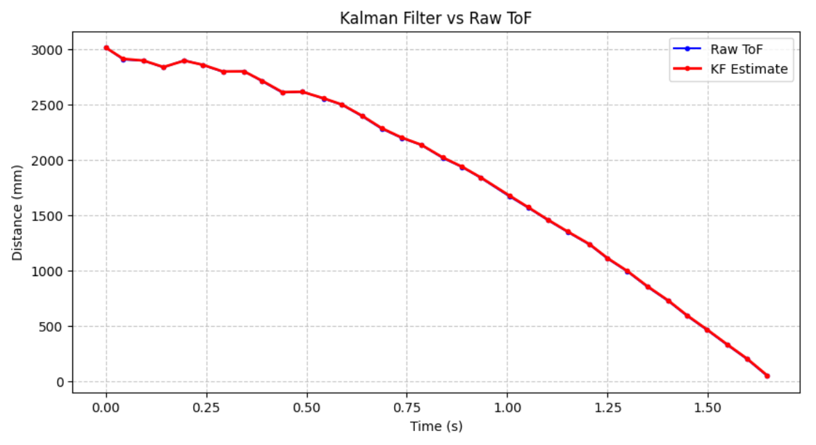 Kalman Filter tested against data sample.
The KF estimate tracks the raw ToF data closely while smoothing out measurement noise. The three covariance parameters collectively determine filter behavior. σ₁ (position process noise) was set to 20mm, consistent with the ToF's specified accuracy, and controls how much the filter trusts its own position prediction. σ₂ (velocity process noise) was set to 158 mm/s, reflecting the high variability observed in the step response velocity data, and allows the filter to update its velocity estimate aggressively when new measurements arrive. σ₃ (sensor noise) determines how much weight is given to each ToF reading, with smaller values causing the filter to snap more closely to the sensor. The values were tuned empirically: σ₃ was reduced from 20mm to 5mm since the ToF performs better than its worst-case datasheet spec at short range with a 50ms timing budget, and the filter was observed tracking slightly above the raw readings at the higher value. σ₂ was increased from 50 mm/s to 158 mm/s to produce smoother diagonal extrapolation between sparse ToF readings rather than stepwise jumps. The final values used were σ₁ = 20mm, σ₂ = 158 mm/s, and σ₃ = 5mm.
Implement Kalman Filter on Robot
The final step would be to actually use this Kalman Filter for our linear PID control from back in lab 5. In order to prepare the code for future use where we would require non-blocking versions of the PID control, new Bluetooth commands were created similar to those used in lab 6, where a flag would be raised indicating the main loop to start running linear PID control. This would allow us to control the robot's distance from walls while performing other tasks concurrently.
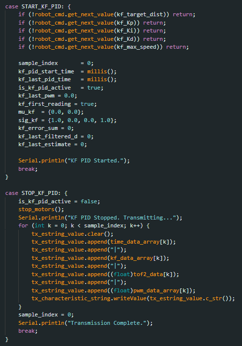 New Bluetooth commands used to start nonblocking linear PID control.
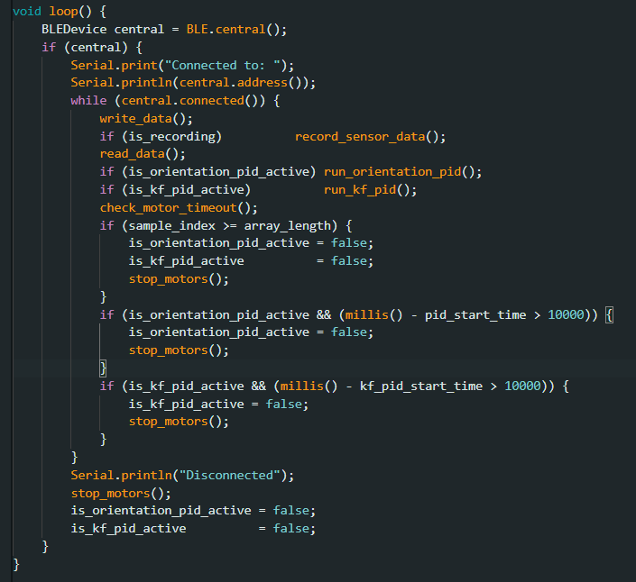 New main loop used to implement the linear PID control.
Our Kalman Filter values were initialized at the top of the code and then used in a helper function just like how we implemented our orientation PID control. Within the helper function itself, the main PWM controls were left nearly untouched from the previous implementations, and the linear extrapolation that we had used before was replaced with our Kalman Filter. As with the extrapolation technique, the Kalman Filter would predict the next distance values, and those would be used for when we would be recalculating the PID control but didn't have any data from the ToF sensor ready.
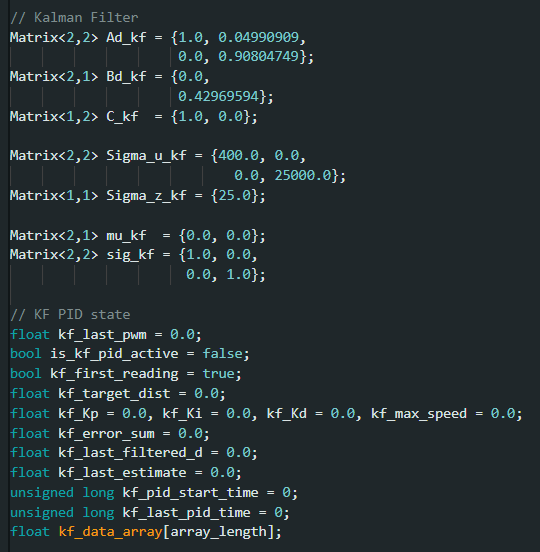 Setting up our constants to be used.
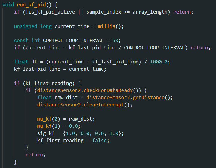
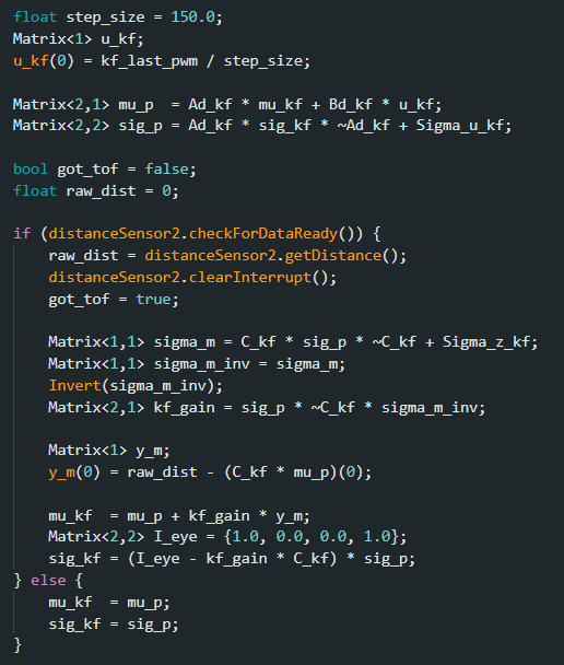
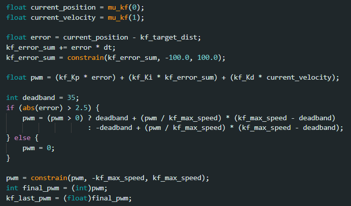 Code used in the new linear PID control.
Even though the Kalman Filter was designed around a specific setpoint of 150 PWM, after initial testing we tried cranking up the speed of the PID control to the maximum of 255, and as seen below, it works very well. The plot comparing the Kalman Filter values and the real ToF data shows the filter effectively estimating the next distance value for the PID loop to use whenever the ToF wasn't ready, leading to a much smoother graph and thus a much more responsive PID loop in general. This is what allows us to have the car be running at maximum speed. Furthermore, it should be noted that, in order to account for the increased, speeds, the specific Kp and Kd constants had to be adjusted to 0.2 and 0.15 respectively to produce good results.
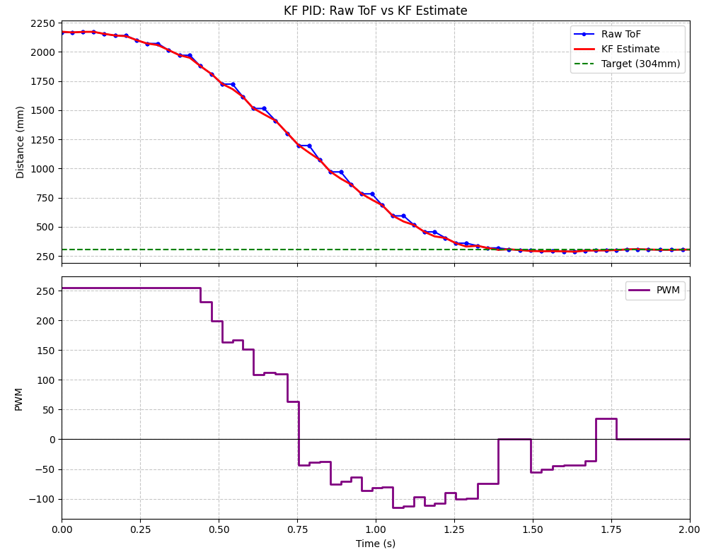 Result of the Kalman Filter vs ToF data showing new smoothed out graph.
Showcasing linear PID control at max speed.
In summary, this lab was very helpful in developing our understanding of Kalman Filters, how to derive them, and their purpose in data collection to help supplement our sensors when our sampling rate might be too low. With this new implementation, we have developed a responsive platform ready to handle the challenges of the next labs. Katherine Hsu's website was used to help inspire elements of this lab.