Prelab
In the fifth lab, we got to fully utilize our new setup that we had completed in lab 4 by implementing a PID control using our ToF sensor to get the robot to reliably and consistently stop one foot before a wall. Throughout this lab we learned about the different ways in which this could be accomplished and certain tricks to help improve performance.
Like with all the previous labs, we made use of the Bluetooth connection that we had already setup beforehand in previous labs to transmit and receive data between our PC and the Artemis board. This would not only allow us to collect data like we had done in previous labs in order to plot out distance to the wall versus time, but we could also setup inputs so that we can easily adjust the different PID variables as we want without needing to reflash the board. See the pictures below for the code.
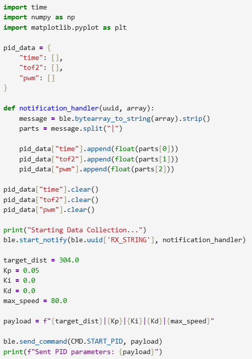 Python side receiving and sending inputs.
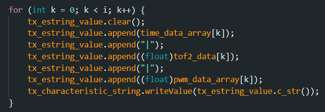 Arduino side sending valuable data.
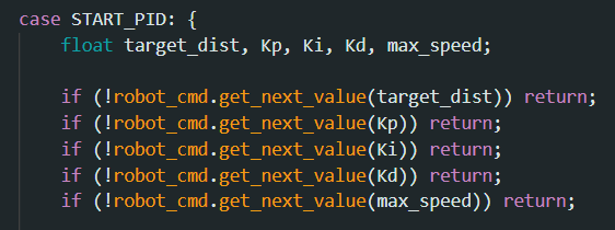 Our new Bluetooth command.
Overall, this setup will make it very easy and convenient for us to test the different values that we'd like to use for our PID control and to plot out the data to see how certain configurations perform compared to others.
Lab 5
Initial Position Control
As mentioned previously, the goal of this lab is to get the car to successfully stop 1 foot in front of a wall. To this end, we will be reusing our code from the previous labs specifically for our ToF sensor. By continuously polling and acquiring data, we will be able to adjust the PWM value of the car's motors to get to the correct location consistently. In short, we will be able to calculate the PWM value of the motor through summing up three different terms as seen in the equation below. Each term has an associated constant which we will need to figure out through testing.
 Main PID Equation determining our PWM output.
Before we could start with the actual implementation of the speed control, several other parts of the code needed to be set in place first. The first key aspect was to set a maximum speed limit so that we could avoid having the car accidentally crashing into the wall at an incredibly high speed. Secondly, knowing the minimum PWM value at which the car could actually move forward, we'd have to scale the output such that the motor could actually react and move the robot. Otherwise, for small movements, the controller would just output a PWM value within our deadband and the car would simply not move. An additional aspect of this part of the code was to set up a limit at which point we would consider the car to be "close enough" to the desired location. A side effect of having this scaling function means that even for the smallest discrepancy, that discrepancy will be scaled up and the car will lurch in whichever direction it's off by. For a value of say one or two millimeters this would just cause the car to overcorrect or constantly keep moving and oscillate, so to correct for this we set an error range such that if the car is within that we will simply stop, ensuring clean stops.
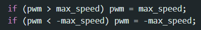 Setting a limit to how fast the car can go depending on the inputted max speed.
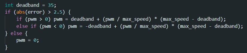 Scaling function used to avoid deadband region of our PWM signals.
The first part and arguably the most important part of the PID control loop is the P, which stands for proportional, where the speed of the car will be adjusted directly in response to how far away it is from the current target. That value, the error, can easily be calculated using the following equation:
 The value that will be multiplied by our Kp.
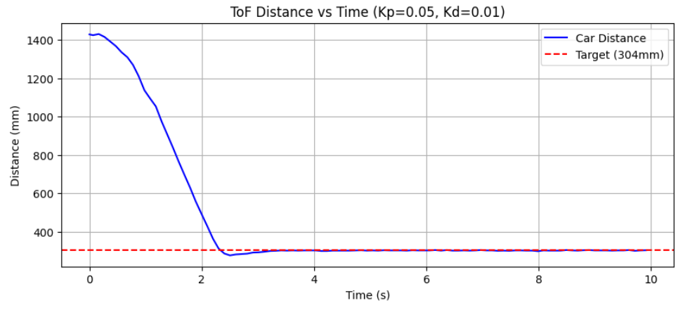
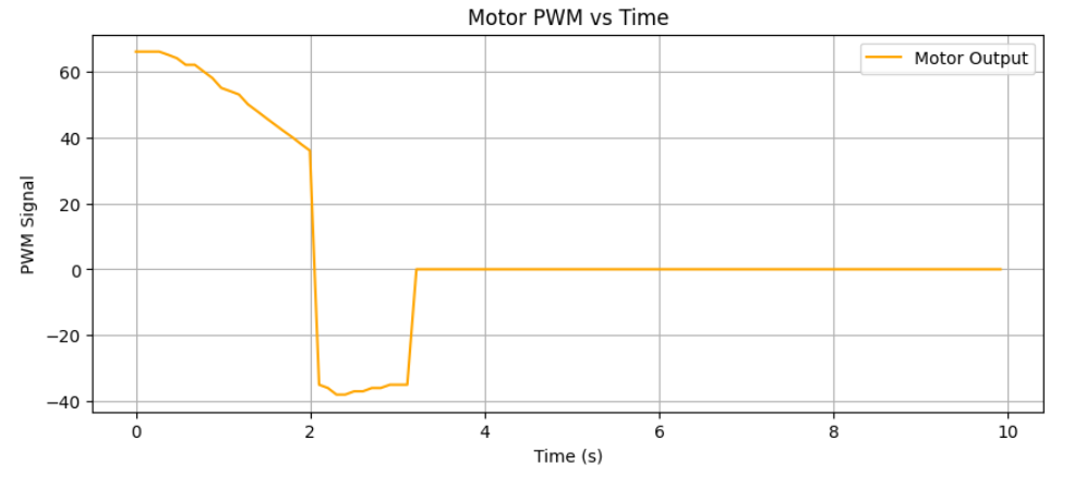
In order to test out finding a good Kp constant, which would determine how the PWM would react to the distance, we cycled through a couple of different values, starting very small since the higher we go then the more the car will overshoot the target and the more likely we will be to have a crash. During this process the Kd and Ki values for the other parts of the PID control were set to zero so that we could fully focus on getting the Kp value correct. When it came to picking the "right" value, we wanted the car to be responsive and quick to reach the target point, so we tended to go higher, even if that meant that we would overshoot. The plan was that through adding the other parts of this controller, we could balance things out. In the end, we came to a value of 0.05 for the Kp constant, which provided a nice balance in terms of getting the car to speed up quickly but also not to the point where it would crash. Shown below is the video of the car being controlled by only the proportional term of the PID control.
Showcasing the car using only the Proportional Term of the PID control.
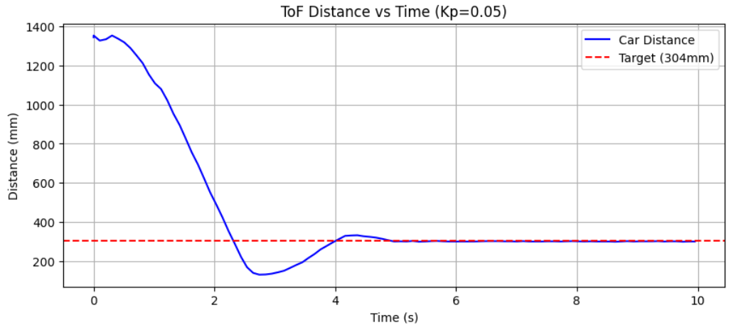 Plot of Distance versus Time.
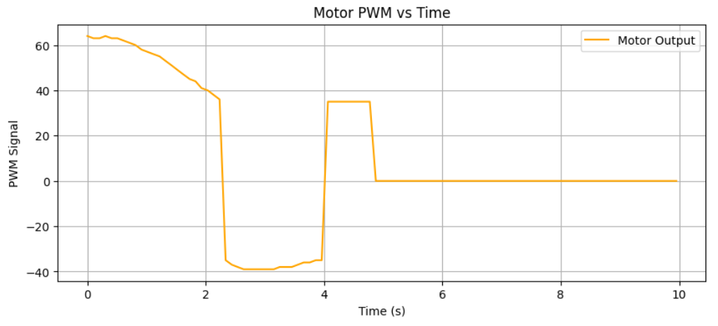 Plot of Car's PWM output Values versus Time.
As shown above, the car overshoots by quite a large margin and even oscillates a little bit between the target point, which is less than ideal, but this provides a good baseline upon which we can build on. Furthermore, it should be noted that due to limitations in the ToF's range itself, it was discovered that the PID control loop only works "correctly" at a maximum range of around 5 feet since further than that and we see the same mismeasurements that were observed in the previous labs, where the ToF sensor would return much lower values than expected. This error would cause the car to still technically move forward towards the target, but in terms of closely aligning to the desired function of the PID control where speed increases the further away the car is, for all intents and purposes the max range is set around 5 feet.
Optimizing Further
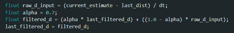
Simply using the Proportional term of the PID control would not suffice as we would overshoot and oscillate, so in order to account for this, next we introduce the Derivative term (D), which adjusts the speed of the car depending on how fast we are approaching the target and helps to prevent the overshooting we observed. The value by which we will multiply the Kd is calculated below. Note that a Low-Pass Filter is implemented in order to reduce noise that would otherwise cause our robot to jitter and oscillate unnecessarily.
 The value that will be multiplied by our Kd.
Now with our Kp value set, we went about getting the optimal Kd value in a similar way, setting everything else constant and testing out various inputs. What we would hope to see when determining the best value is that the car overshoots by just a little. This overshooting indicates to us that the car is at its limit in terms of speed because otherwise if we set the Kd value really low, we wouldn't overshoot but we would approach the target really slowly, which is not what we're looking for. In the end, we found a nice balance at a Kd value of 0.012. Below are our results which demonstrate how much better the response of the car is now with this extra term.
Showcasing the car using the Proportional and Derivative Term of the PID control.
 Plot of Distance versus Time.
 Plot of Car's PWM output Values verus Time.
A small issue that was observed when initially testing this term was the car immediately starting at the maximum speed at the start of the test, which had previously never happened. This was discovered to be caused by what is known as the derivative kick, where, because our earlier point of reference is technically starting from zero velocity, the car believes that the change in speed is extraordinarily high and thus the output is the max. Naturally, we would like to avoid such behaviour as it prevents the car from reacting as it should at the start, so the first time that we run this loop the "last value" is manually set to what is currently seen instead of zero.
The last term in the PID control is our I (or Integration), which helps to reduce any steady-state error that might not be resolved by our current setup. The longer the car is off the target the more this term will affect our PWM output. The equation below was used to calculate the term that would be multiplied against our Ki constant, and it simply just kept track of our error over time. As a necessary safety measure we needed to add wind-up protection to this integrator since the robot would generally be very sensitive to it and we want to avoid the robot making sudden movements out of nowhere. The implemented clamps helped to mitigate this risk. Since the effects of the Ki term can be a bit more subtle compared to Kp and Kd, less testing was done to try to figure out the "best" value and we settled on a safe 0.001, which is small enough that we could prevent low-frequency oscillation of the car when it was near the target.
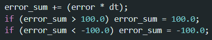 The value that will be multiplied by our Ki.
Extrapolation
Originally, we had been using a blocking version of the PID loop which simply waited for the ToF sensor to return a new value before proceeding with our calculations. However as seen previously this sampling rate is very slow compared to how fast the Artemis could run in general, meaning that we would be losing a lot of potential responsiveness. As a result, the Bluetooth command was changed so that the checking of the ToF sensor would be nonblocking as was done in the previous lab with the ToF. In its place, if we didn't receive a new ToF sensor value, which would happen more often than not due to the high frequency of the main loop, the distance value would simply be extrapolated using the previous two values that were read by the ToF sensor. This would theoretically provide us with more accurate data at any given time, allowing the PID controller to be more accurate when determining what the PWM output should be. Using data acquired with this new loop we could then determine the PID loop frequency versus the ToF sampling rate (see the picture below), and we can also plot out how the raw and extrapolated data compare. Note that the extrapolated data is what is being used for the robot now, and with this higher frequency of data, we would expect the robot to be a lot more accurate in its response, which seems to be the case (doesn't overshoot anymore).
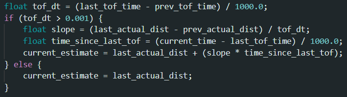 Math used to calculate extrapolate the next distance measurement.
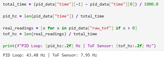 Math used to calculate the sampling frequency.
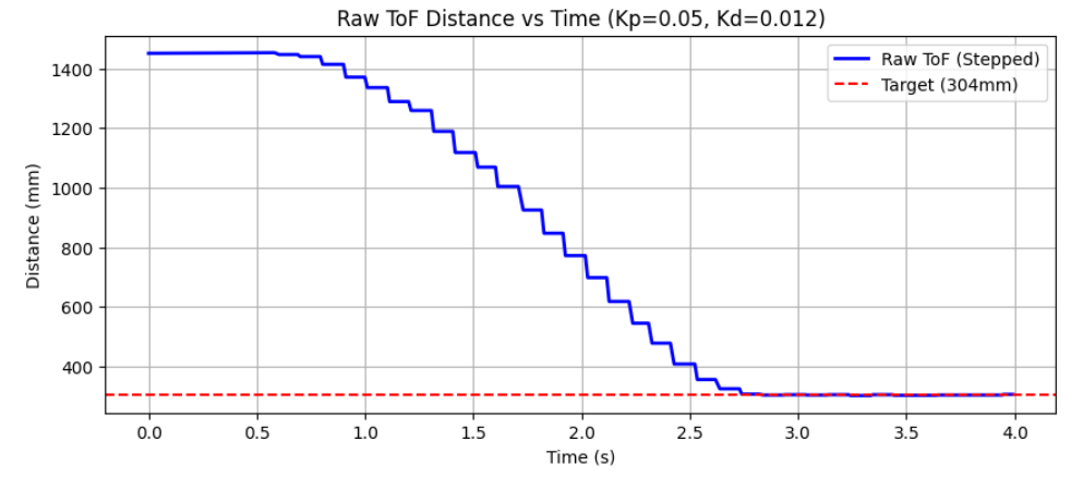 Plot of our raw data.
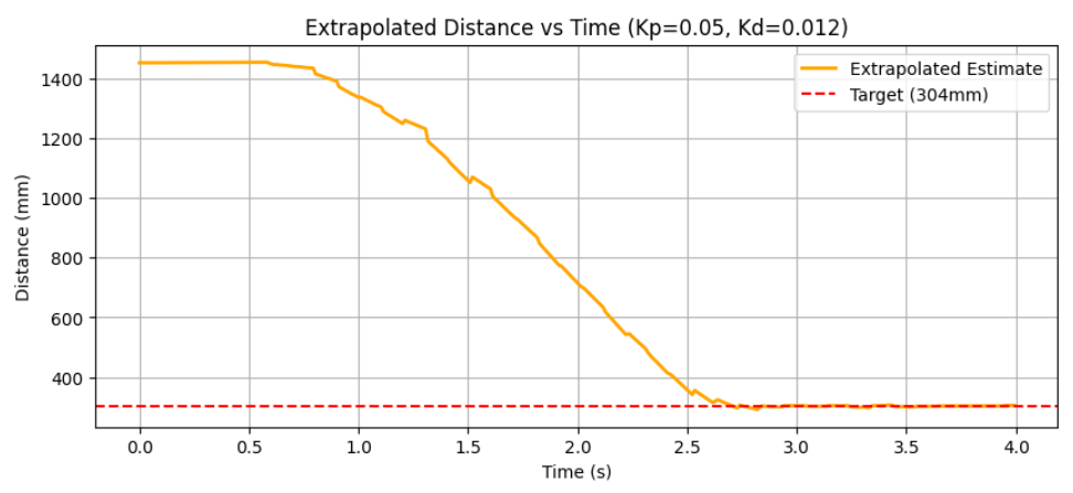 Plot of our smoother extrapolated data.
Demo
Putting all the pieces together, shown below are three demos of the car starting from different positions, including in front of the target area, showing how it reliably and accurately stops at the one foot mark. For the trial where the car starts from the farthest point, the maximum speed was set to a limit of 255 to see what the max linear speed was, and, using positional data, it was calculated to be around 0.45 m/s, which is a bit slow but could perhaps be increased further if the car had a better sensor capable of measuring longer distances. Overall, the implementation of the PID control was a success, and a lot of insights were gained in how different mathematical models were used to help better control the car's behaviour.
Three Demonstration Videos Showing the Car from Different Starting Positions.
Katherine Hsu's website from SP25 was used to help inspire elements of this lab.