Prelab
In the third lab, we learned how to use our Time of Flight (ToF) sensors, testing and configuring two different sensors in order to simultaneous collect distance data.
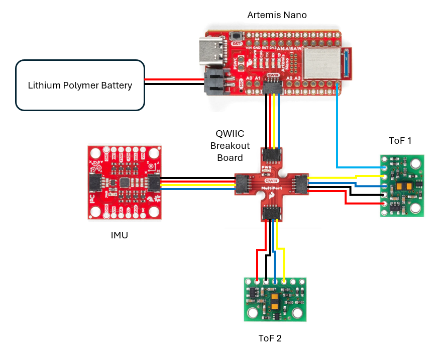
To begin the lab, we would first need to understand how the ToF sensors would need to be wired to the Artemis Nano and then have connections soldered accordingly. Using the datasheet, we can determine that the blue wire on our connectors represents SDA while the yellow wire represents SCL for the I2C connection. The two ToF sensors, IMU, and the Artemis Nano would all have their power, ground, and I2C wires shared, with a QWIIC Breakout Board splitting the wires in between the four boards. Additionally a battery would be soldered to a JST connector that is compatible to the Artemis Nano, meaning that we will be able to power the board without the USB connection to the laptop that we've been using up to this point. A concern was a possible misalignment of the power and ground wires with the correct wire colour (red to black and black to red), but fortunately that wasn't an issue in our case.
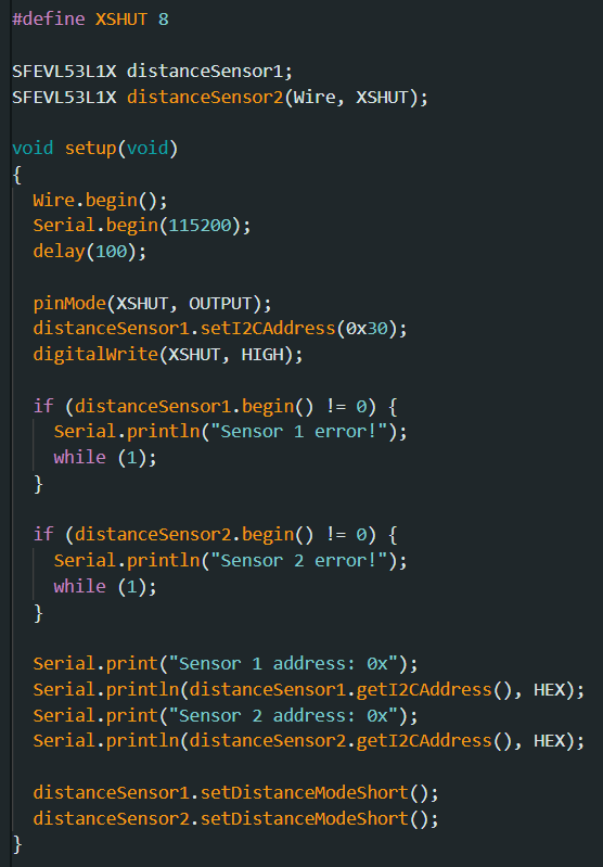
The Artemis Nano would know from which board it would be receiving data by knowing their specific address. Using the datasheet, we know that the ToF sensors have a default address of 0x52. However, maintaining this for both sensors would cause problems in the future since we wouldn't know what data is coming from which sensor. Therefore, we will need to change the address, and that will be accomplished through soldering an extra connection between one of the sensor's XSHUT pins to a GPIO pin on the Artemis Nano (will be discussed in a later section). Shown below is a wiring diagram of our setup.
 Wiring Schematic of Our Setup.
The plan for the the sensor placement will be at the front and on the side of the car (most likely on the right). This is facilitated by the current connection of our sensors as was shown in the wiring diagram, with the two sensors being rotated 90 degrees from one another. The intention is to be able to observes obstacles directly in the way of the car and also to the side. We will be therefore be lacking coverage of the areas 1) above the car itself (irrelevant), 2) behind the car (unlikely to have obstacles as long as we're not reversing), and 3) to the side of the car without the sensor (can still be detected through rotation). Additionally, since we want to maximize future flexibility with the exact positioning of the ToF sensors (the IMU and Artemis Nano themselves can be centrally placed), the longer QWIIC connector cables were soldered onto them.
Lab 3
Picture of ToF Sensor Connections
 Picture of Entire Wiring Setup.
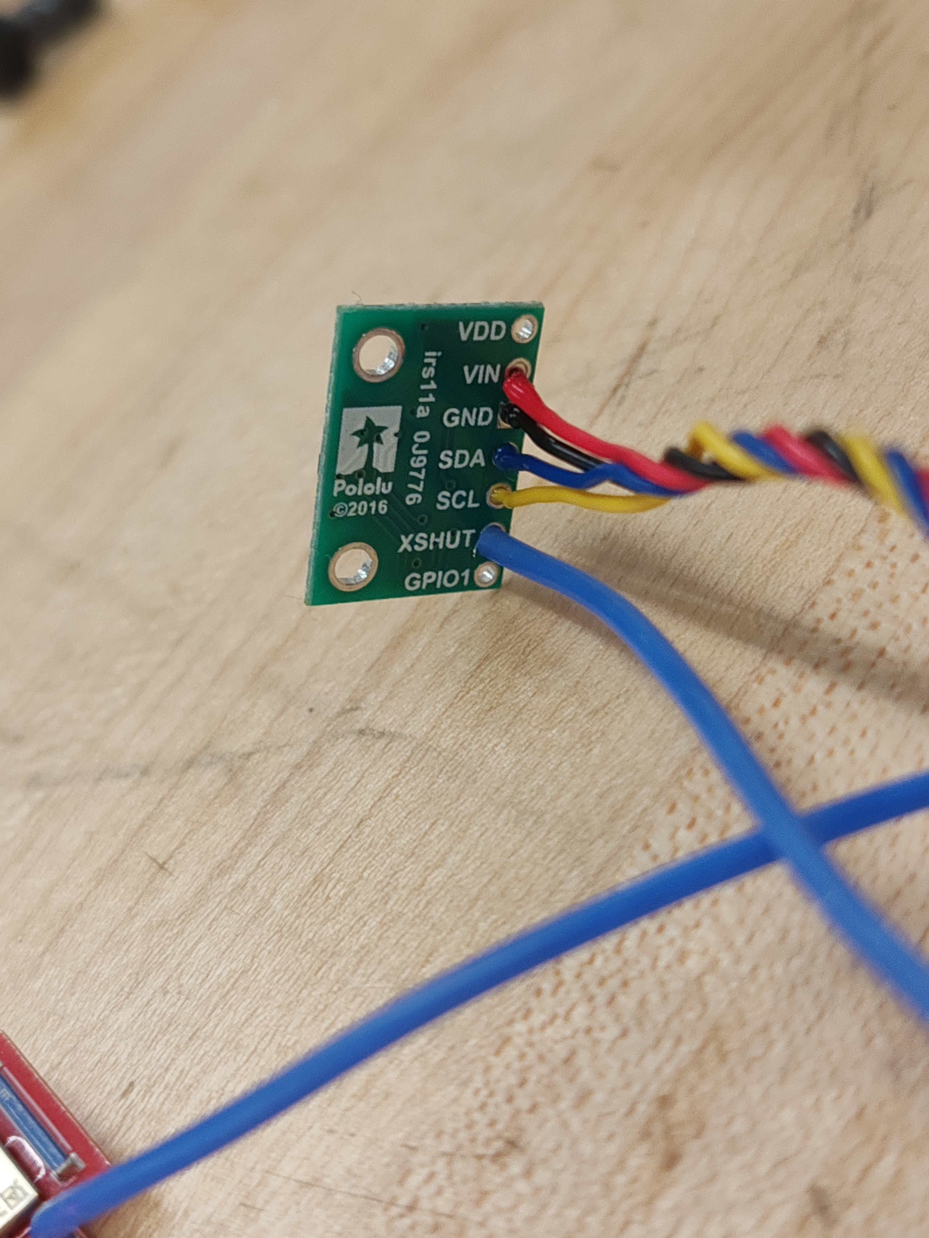 Picture of ToF Soldered Connections.
Artemis Scanning for I2C Device
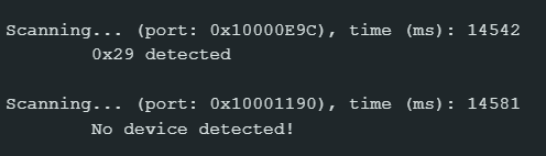
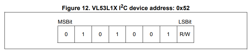
As shown in the picture below, a device is detected at address 0x29 when just connecting one ToF sensor to the breakout board. This is surprising since the address we would expect to appear would be 0x52. However, this is simply just the same value shifted right by one bit. According to the datasheet (also shown below), the LSB of the address is used to indicate whether or not we're reading or writing. Therefore, the output matches our expectations.
 Printed Result of I2C Example Code.
 ToF Datasheet showing the Address.
Testing Distance Sensing
The ToF sensor has three modes: short, medium, and long. According to the ToF datasheet, the long distance mode allows for the longest possible ranging distance of 4 meters to be achieved, but that limit is pretty heavily impacted by ambient light. On the other hand, while the short distance mode has a more limited ranging distance of 1.3 meters, it is more immune to ambient light. Therefore, considering the fact that there will almost certainly be strong ambient light for all future uses of the sensor, the short distance mode was selected.
In order to test the sensor itself, it was setup as shown in the picture below attached to the laptop to ensure it was facing a relatively close to parallel to the ground. A measuring tape was setup with a box that would be move across several distances to compare the sensor's reported distances with the actual real values. It should be noted that some error would definitely be present due to slightly imperfect orientation of the measuring tape and the laptop, causing the actual "real" distance to be greater than what was noted down.
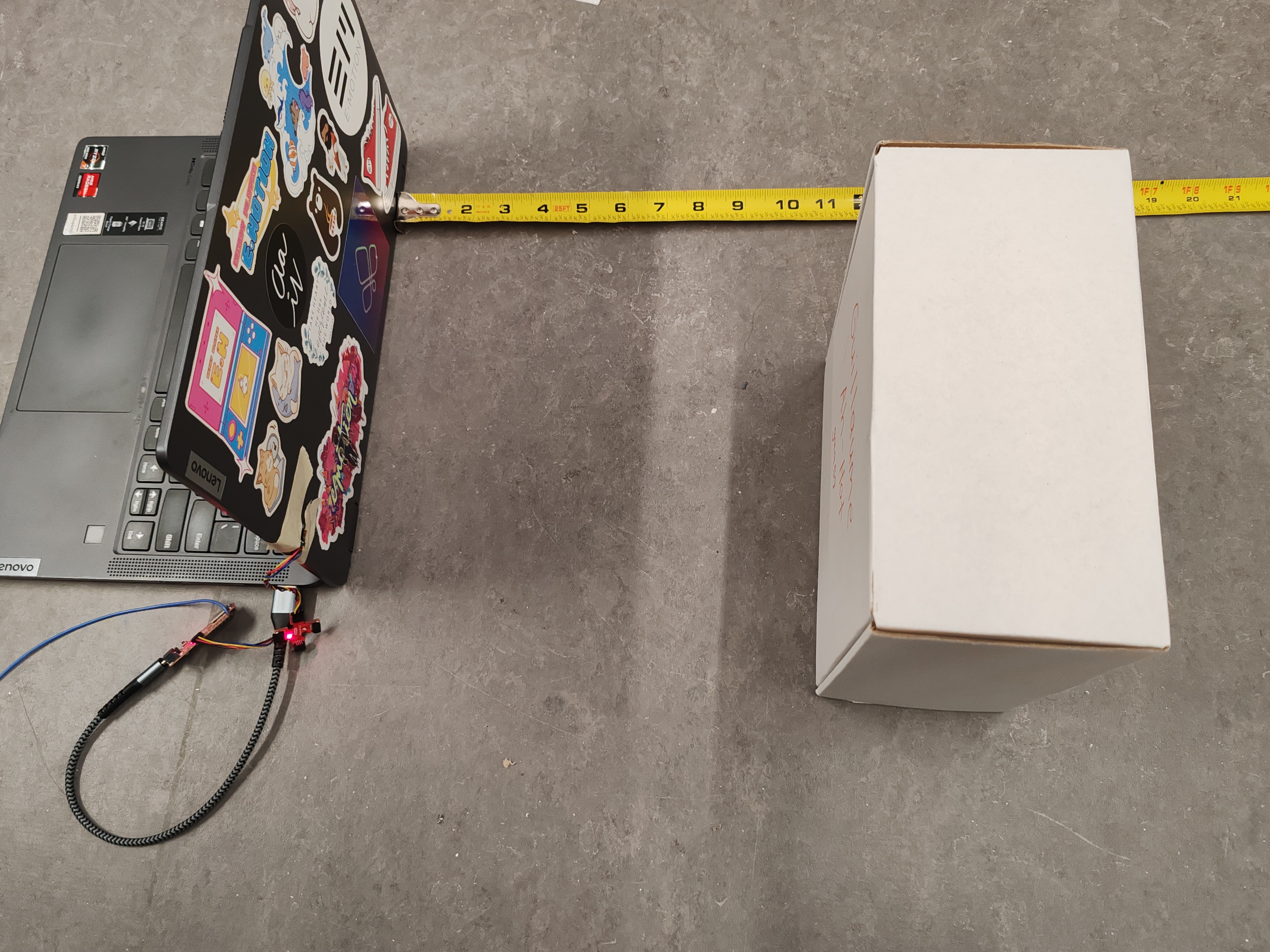 Image of Setup used to collect Distance Measurements.
Shown below are the results of our data measurements. The code used to collect data was based the example code that came with downloading the SparkFun VL53L1X 4m laser distance sensor library, with some adjustments for convenience and also the use of the millis() function in order to record the time each loop took.
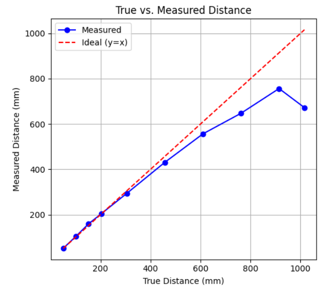 Plot of Recorded vs True Distance Measurements.
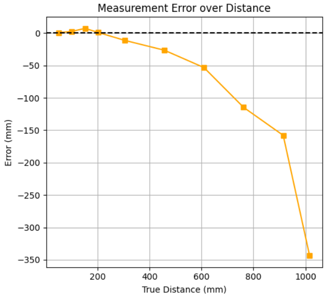 Plot of Recorded Data Error Compared to Real Values.
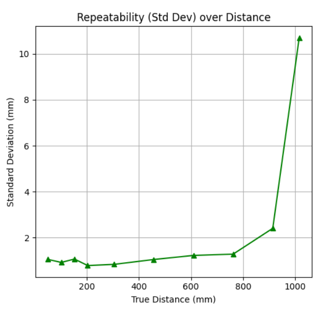 Plot of Deviation of Data for Each Distance Point.
As seen in the plots, as the real distance increases, the ToF sensor begins to increasingly return values below the expected value. This comes to a head after ~900mm where the sensor begins to fail entirely and starts reporting garbage values, which is significantly below the expected maximum range of 1.3 meters that was described in the datasheet. As expected, along with an increasing rate of error, the standard deviation of the data collected for longer distances also grows. However, the magnitude of the discrepancies themselves is still small enough (a couple of millimeters) where we can be relatively confident in the repeatability of the sensor before it reaches its maximum range. While the sensor could potentially detect the existence of obstacles past 900mm, the distance value would be so far off the true value that the only useful case would probably if the car was travelling very fast and needed to detect the presence of a wall/obstacle in front of it fast enough to successfully evade it or stop. However, for any other case where we would need a somewhat accurate reading, we would probably set the maximum range to approximately 900mm. Additionally, after measuring the time it took for ranging, it was very surprising to see an extremely consistent value of 50ms across all distances. There was no variation at any point, which is positive news since this means we can confident in the consistency of the ranging time.
Two ToF Sensors in Parallel
As mentioned previously, an extra wire was soldered between the GPIO pin 8 of the Artemis Nano and the XSHUT pin of one the ToF sensors. This is important as it allows us to effectively turn that ToF sensor off so that we may change the I2C address of the other ToF sensor. Otherwise, trying to change one ToF sensor's address would end up changing both since they default to the same starting address. The code below shows how we setup the two sensors: turning off one sensor, changing the active one's address (to 0x30), and the switching back on the other sensor.
 Setting up the I2C addresses of the two sensors.
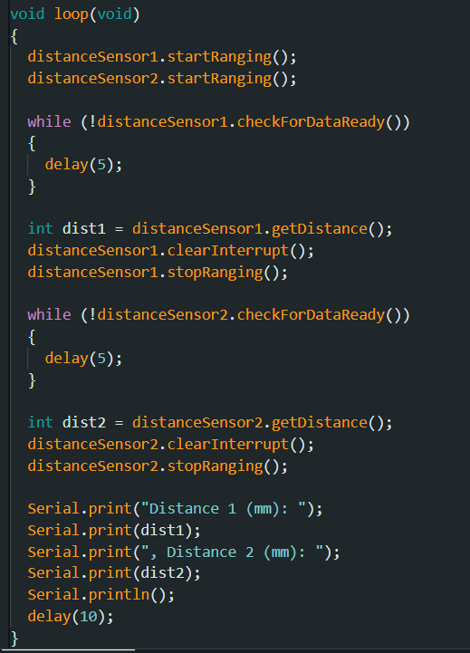 Code to collect and print the data of both sensors.
Showcasing both ToF sensors working in parallel.
ToF Sensor Speed
In order to accurately measure the speed of the ToF sensors, a new loop was created that would continue looping and printing the time, only printing the distance values when they were ready using the checkForDataReady() function. Key to making this loop as fast as possible was to move the startRanging() command to the setup function, meaning that we would only have to perform it once instead of every loop like how it was before. The following snippet of the output below shows a difference of around 99 milliseconds between two measurements from the same ToF sensor while one loop itself took 5 milliseconds, a difference of almost 20 times. This shows that the sensors themselves can't keep up with the rate at which the serial monitor could theoretically print outputs, so in this case the limiting factor in our ability to transmit data isn't the serial monitor's ability to print (or anything to do with the baud rate), but limitations with the sensors.
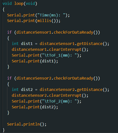 Code of revised nonblocking loop to collect distance measurements.
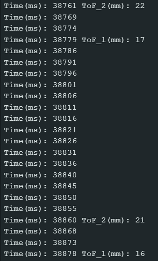 Output of Serial Monitor.
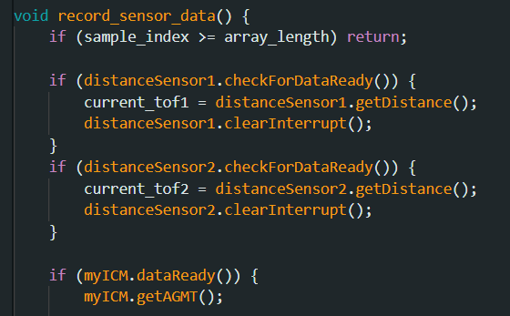
Combining ToF and IMU Data
Conveniently building on work done in the past weeks, all that's required for this part is by adding several arrays and lines to our existing code, specifically the get_IMU_data() function that we had previously, which is now transformed into record_sensor_data(). As shown below, with the understanding that the IMU is able to collect data at a much quicker rate than the ToF (calculated ~64 Hz sample rate for IMU last lab), we need to avoid blocking the function to wait for the ToF to receive data. Using a similar setup as in the previous section, the code will not wait for the ToF sensors to return data, but instead just use the previous value if no new data is ready. Due to this discrepancy in sampling rates, the plots for the ToF sensors and the IMU look very different, with the former being a lot less smooth than the latter. This setup, however, ensures we receive the most up-to-date data at any given point.
 New nonblocking code.
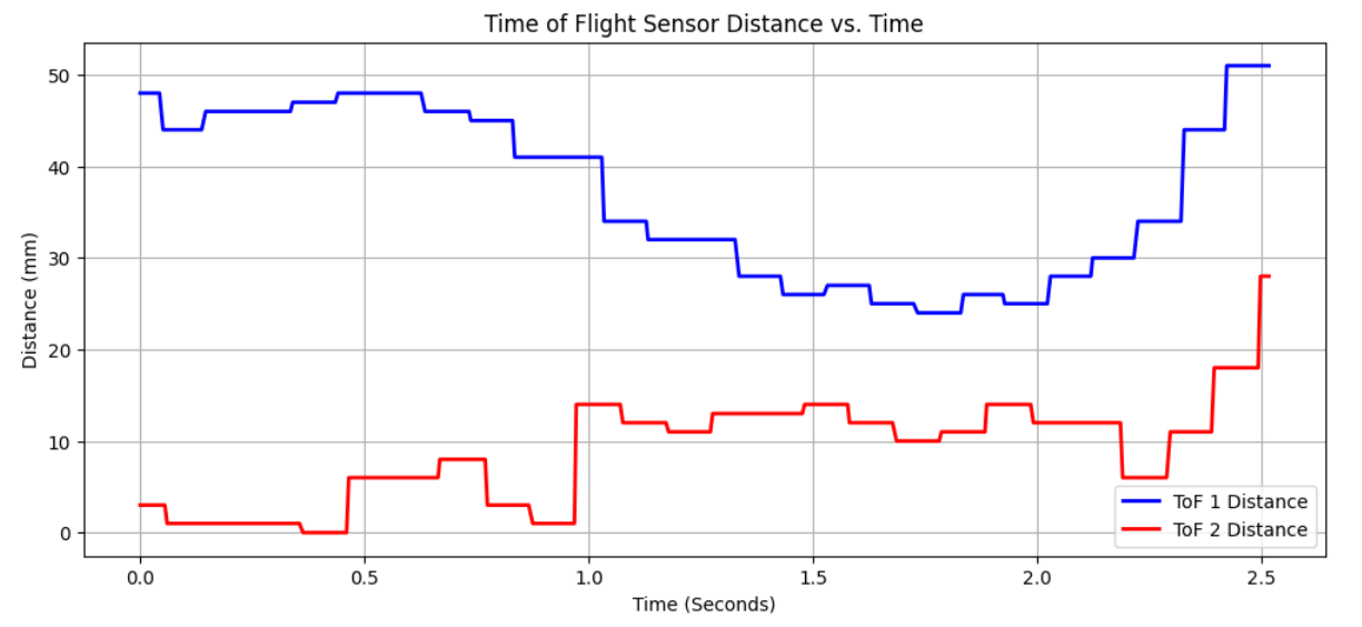 Plot of ToF sensors showing low sampling rate.
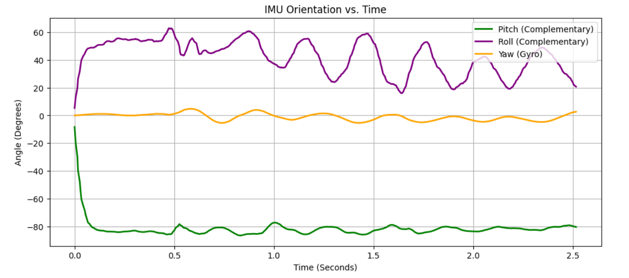 Plot of IMU showing higher sampling rate and smoother curve.