Lab 2: The IMU
Reading and Filtering Accelerometer / Gyroscope Data
1. Setup the IMU
In the second lab, we learn how to collect and process data from an Inertial Measurement Unit (IMU) connected to our Artemis Nano microcontroller, applying filters to pitch and roll information drawn from the IMU's accelerometer and gyroscope to help remove noise.
To begin the lab, I installed the “SparkFun 9DOF IMU Breakout_ICM 20948_Arduino Library” from the Arduino Library Manager and connected the IMU to the Artemis Nano using the QWIIC connector. This step would allow us to test out example code to verify the IMU's functionality. By running Example1_Basics, we can observe a set of information being repeatedly printed out on the Serial Monitor, including accelerometer and gyroscope data.
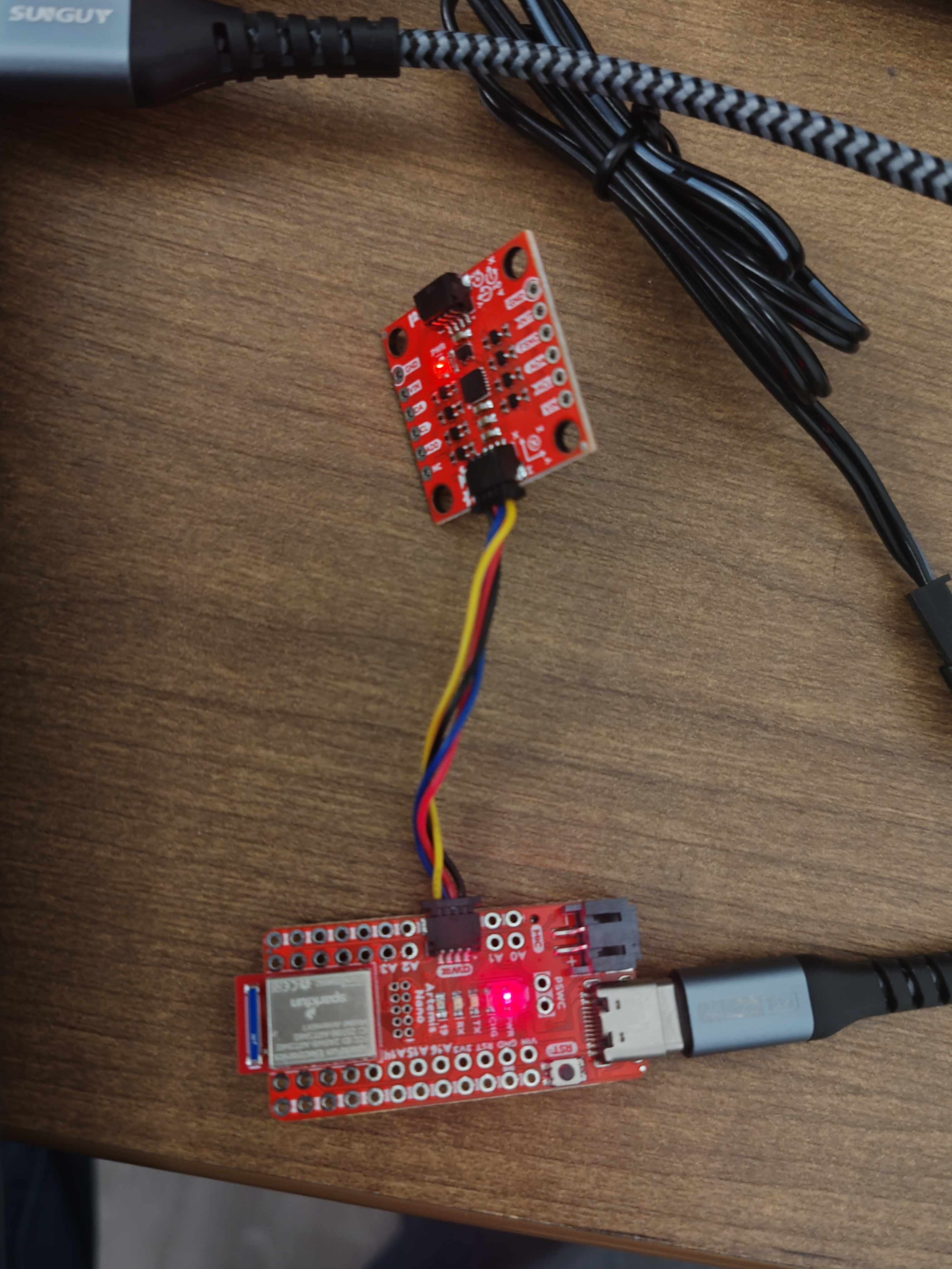 The IMU connected to the Artemis Nano via QWIIC.
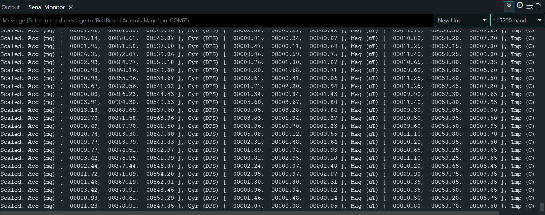 Output of Running Example IMU Code.
AD0_VAL Definition
In the example code, the AD0_VAL definition represents the value of the last bit of the I2C address. On the SparkFun breakout board, the ADR jumper is open by default, which corresponds to a value of 1. If we were to solder this jumper closed, the value would be 0. This feature is significant because it allows us to connect two identical IMUs to the same I2C bus without address conflicts (one set to 0, one set to 1).
Acceleration & Gyroscope Data
By running the example code and observing the raw sensor data, we can very quickly check if the reported information is as expected:
- Accelerometer: The accelerometer section prints out the magnitude of acceleration in the X, Y, and Z directions. When the board is sitting flat on the table, the Z-axis reads approximately 1000 mg (1g) with the X and Y axes near zero. This makes sense considering only the Z-axis in this case is aligned with Earth's gravity, and further tilting the board caused changes, reflecting how gravity's pull in the different directions shifted.
- Gyroscope: When the board was stationary, the values fluctuate slightly around 0. These values spike significantly once the board started rotaing, reflecting the angular velocity (degrees per second).
Visual Feedback (LED Blink)
To provide a visual indication that the IMU has initialized successfully and the code is running, I added a startup sequence that blinks the onboard LED three times.
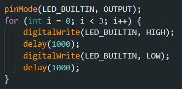 Code added to initial startup for visual feedback.
LED blinking on startup.
2. Accelerometer
The accelerometer measures linear acceleration (including gravity). By analyzing the gravity vector, we can compute the pitch and roll of the board.
1. Pitch and Roll Calculation
Using the equations shown in class, I converted the raw accelerometer data into angles. I implemented a helper function get_pitch_roll containing these equations to calculate this data and then print_pitch_roll in order to quickly check our values:
Pitch & Roll Equations
pitch = atan2(accX, accZ) × 180 / π
roll = atan2(accY, accZ) × 180 / π
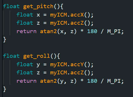 Code containing pitch and roll equations.
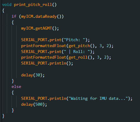 Code to print out pitch and roll data for easy observation.
2. Two-Point Calibration
To check the accuracy of the accelerometer, I placed the IMU on a flat surface and rotated it to -90, 0, and 90 degrees. As shown in the video below, the sensor output appeared to be quite close to what was expected. While difficult to get a "correct" measurement of 90 or -90 degrees from placing the IMU upright against the table, the most consistent and easily verifiable part of this test was laying the IMU flat against the surface. As shown in the video, pitch and roll when the IMU was flat neared zero degrees, which showed that there was very little baseline skew at the very least within the IMU's readings. This observation led me to conclude that applying two-point calibration would not be necessary.
Verifying Pitch/Roll accuracy at different orientations.
3. Noise Analysis (FFT)
Accelerometers are inherently noisy and susceptible to mechanical vibrations. To analyze this, I recorded data under three conditions: 1) with the IMU stationary to measure baseline noise, 2) with the table shaking to simulate motor vibrations expected in the future, and 3) with the IMU being actively moved and rotated around. This assortment of conditions would provide good variety that would supply us with the different kinds of frequency readings that we would need in order to properly define a cutoff frequency for our low pass filter. Shaking the table for example would help us get a lot more high frequency data points while the rotating the IMU around would provide low frequency data points.
I used the Python script below to perform a Fourier Transform (FFT) on the collected data, which was based on the example provided in the lab instructions. This allowed me to visualize the frequency spectrum and distinguish between the "good" low-frequency data (actual tilting) and the "bad" high-frequency noise (vibrations).
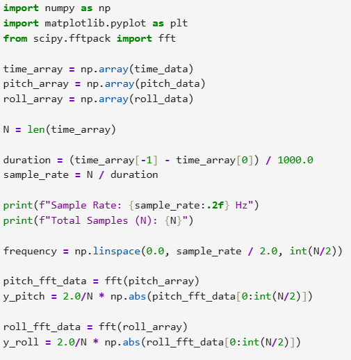 Python code used to calculate the FFT.
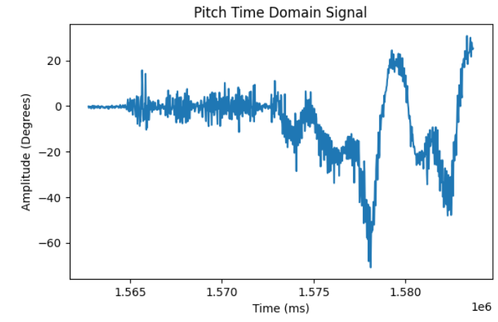 Pitch data in Time Domain (Raw).
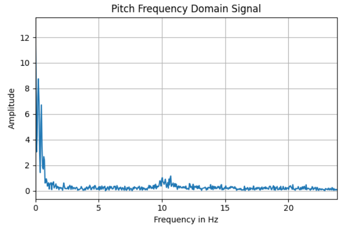 Pitch data in Frequency Domain (FFT).
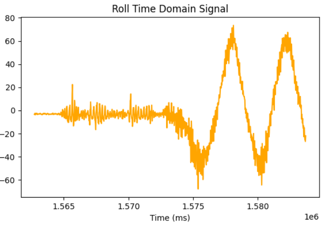 Roll data in Time Domain (Raw).
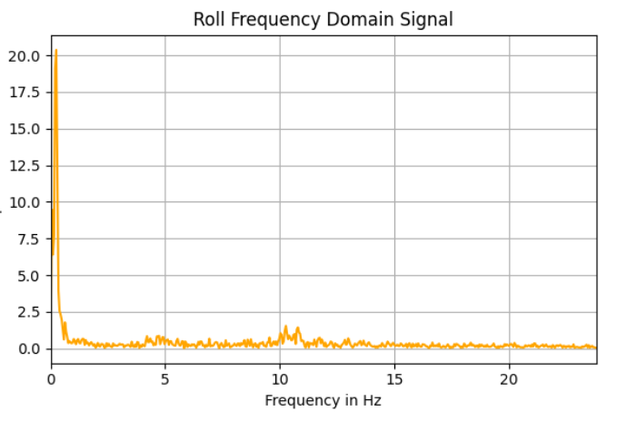 Roll data in Frequency Domain (FFT).
The FFT graphs show a slight bump in amplitude around 10 Hz, likely corresponding to mechanical noise. To effectively filter this out while keeping the board responsive, I chose a cutoff frequency of 5 Hz.
4. Low Pass Filter (LPF) Design
To implement the filter, I first calculated the sampling rate of my loop. As shown in the screenshot below, the loop runs at approximately 47.67 Hz.
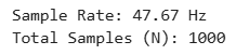 Measured sampling rate of ~47 Hz.
Using the sampling rate (Ts ≈ 0.021s) and my desired cutoff frequency (fc = 5Hz), I calculated the smoothing factor α:
Low Pass Filter Calculation
RC = 1 / (2π × fc) = 1 / (2π × 5) ≈ 0.0318
α = Ts / (Ts + RC) = 0.021 / (0.021 + 0.0318) ≈ 0.4
I implemented this filter in the Arduino code as shown below:
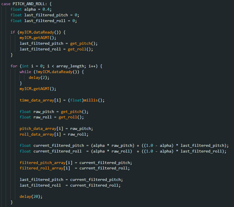 Code snippet implementing the LPF logic.
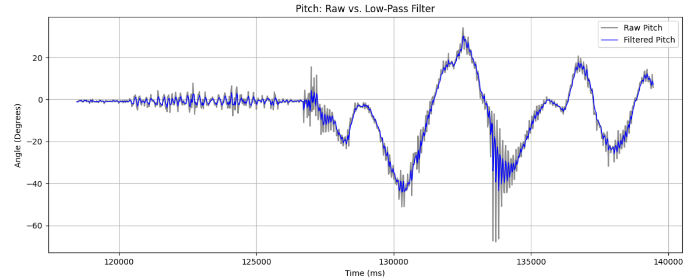
The plots below compare the raw accelerometer data (blue/orange) with the filtered output (overlaid). The LPF successfully reduces the amplitude of the high-frequency oscillations (noise) while tracking the general motion of the IMU.
 Pitch: Raw vs Filtered.
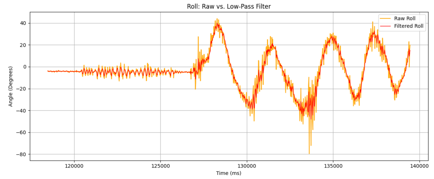 Roll: Raw vs Filtered.
3. Gyroscope & Sensor Fusion
While the accelerometer calculates orientation using gravity, the gyroscope measures angular velocity (ω). To get the actual angle (Pitch/Roll/Yaw), we must integrate this velocity over time:
Gyroscope Integration
θnew = θold + (ω × dt)
1. Drift vs. Noise
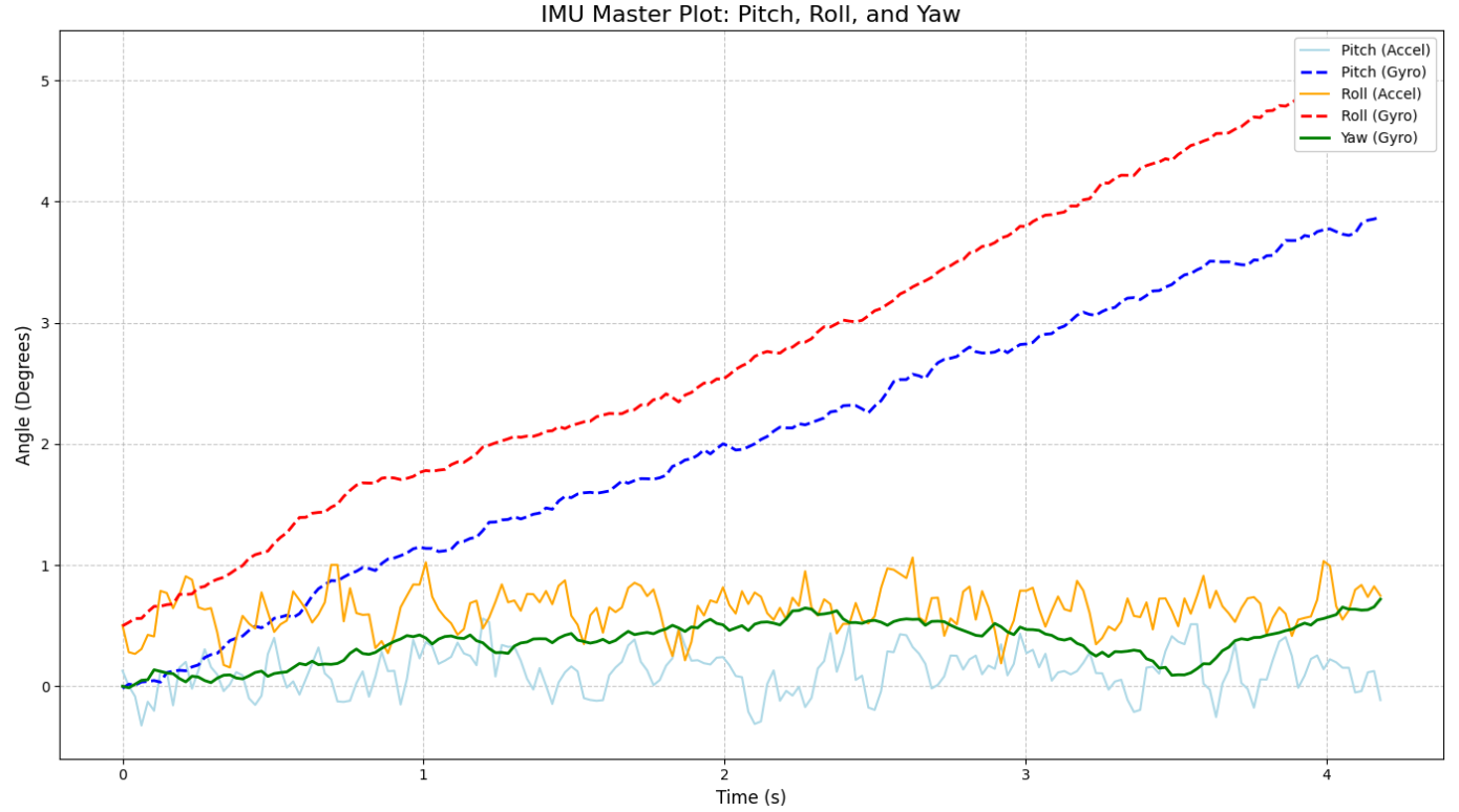
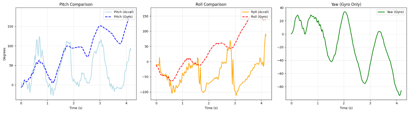
The plots below compare the angles derived from the Accelerometer (Light Blue / Orange) versus the Gyroscope (Dashed Blue / Dashed Red / Green) under different conditions.
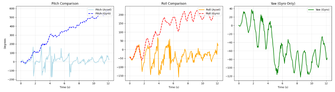
- Stationary: When keeping the IMU still on the table, the accelerometer is noisy (despite implementing the LPF) but the output remains flat and consistent over time. On the other hand, the gyroscope is extremely smooth (low noise) but slowly drifts away from 0 due to tiny errors accumulating in the integration, leading to massive discrepancy after several seconds.
- Moving: When slowing tilting and rotating the IMU around, the gyroscope tracks the rapid movements perfectly without the "jitter" seen in the accelerometer data, but unfortunately, there is still the same drift seen in the first example, and eventually after a couple of seconds there becomes large offset.
 Stationary: Note the gyro drift over time.
 Moving: Gyro is smooth but offset.
2. Effect of Sampling Frequency
To test the importance of a fast sampling loop, I artificially added a delay (changing delay(20) to delay(60)) and redid the the test with moving the IMU around. As shown in the plots, there is a similar offset that grows after a couple of seconds as seen before, but looking at the y-axis, it becomes immediately clear that the magnitude of the discrepancy has effectively multiplied compared to when the delay was shorter before. This happens because integration relies on the assumption that the angular velocity is constant during the time step dt. When dt becomes too large, we miss the nuances of the motion curve. A sudden spike in velocity might happen entirely between two samples, causing the integration to "underestimate" the total rotation, leading to massive drift.
 Gyroscope integration error with slower sampling.
3. Complementary Filter
To get the best of both worlds, I implemented a complementary filter. This fuses the signals by acting as a high-pass filter for the gyroscope (trusting it for fast changes) and a low-pass filter for the accelerometer (trusting it for long-term stability).
Complementary Filter Formula
θcomp = (α × (θcomp + ω × dt)) + ((1 − α) × θacc)
Implementation of Gyro Integration and Complementary Filter.
I selected an alpha value of 0.8. This means the filter relies 80% on the gyroscope and 20% on the accelerometer at each step. This value provided a good balance: it was high enough to smooth out the accelerometer's vibrations but low enough to correct the gyroscope's drift quickly. As shown in the plots below, the recorded data received is not only smooth but stays consistent over time.
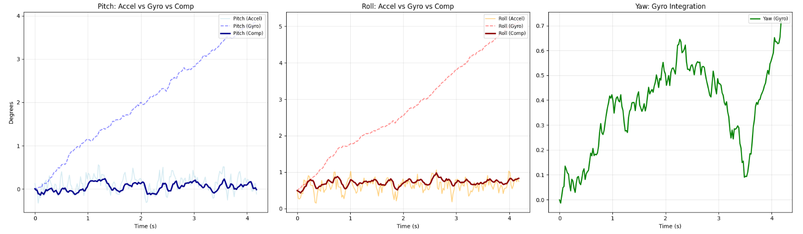 Filter eliminates gyro drift while stationary.
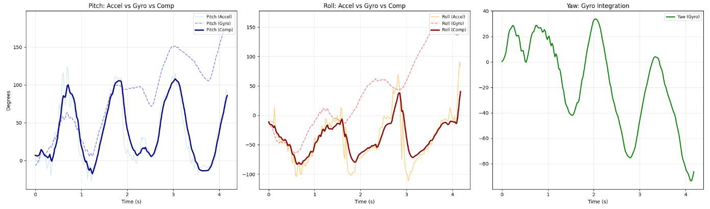 Filter tracks motion smoothly without noise.
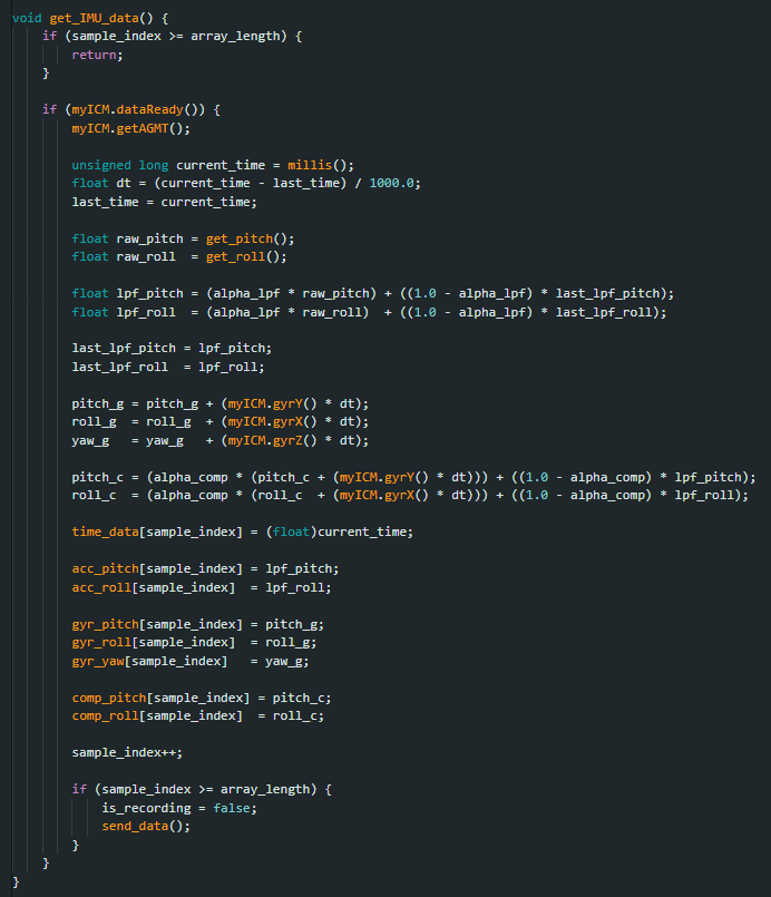
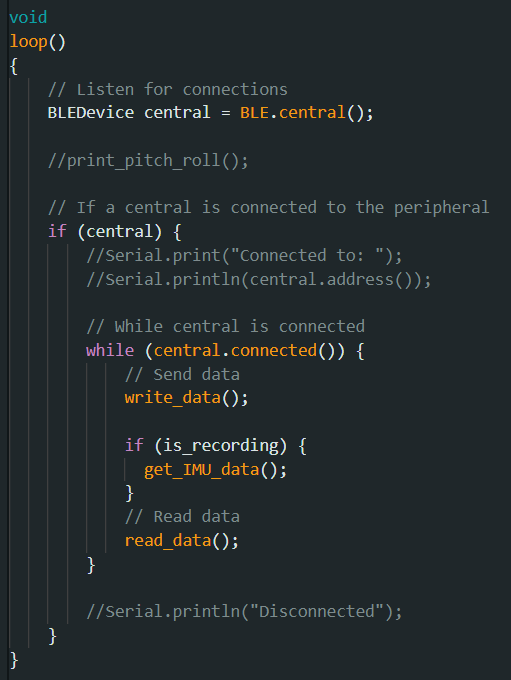
4. Sample Data & Speed
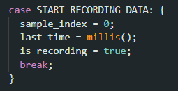
As shown in the pictures of code below, a new implementation of the data collection was set in place, where sending a command would set high a flag which would indicate in the main loop to start collecting data. This would allow us to continuously receive data values from the IMU where we could then use on the Python side.
As instructed in the lab manual, I removed all delay() calls and Serial.print statements from the main loop in order to try to speed up the data collection as much as possible. I used a single array to store the output data as that would help simplify having the synchronize gyro and accelerometer data with time on the Python side of the code while also potentially saving memory from not needing to have multiple arrays. I used a float data type in this case in order to allow for higher precision of data collection and calculation for the angle values we might receive. which would be important when calculating values such as derivatives.
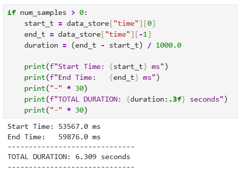
I set the array size to 400 samples. As shown in the picture, we have a collection time of 6.309 seconds (satisfying the >5s requirement), meaning we have a sample rate of approximately 63.4Hz. Given the fact that we store 8 floats (4 bytes each) for every sample, that means one sample of measurement takes 32 bytes. With our memory size of 384kB, this leads us to an absolute maximum of total of around 12,000 measurements that we could theoretically store (though the real number is very likely lower). Using the previously calculated sampling rate, we would be able to capture data for approximately 189.3 , or just over 3 minutes, which is quite good.
 Command to start collection.
 Helper function called in main loop.
 Adjusted main loop.
 Python console output confirming >5 seconds of data received.
5. RC Stunt
The video below showcases some of the RC car's capabilities. After playing around for a bit, it was observed that the car's controls were very sensitive, meaning that trying to align the car in a specific direction was quite challenging. The car's rotation speed was fast, allowing it to make very quick turns, and the max speed was also quite high. Most interesting though would be the car's ability to effectively flip on its back and still drive properly, so one of the cooler tricks would be to have the car roll against the wall and flip upside down.
Driving the RC car.