Overview
The purpose of this lab is to implement grid localization using a Bayes filter in simulation. Pure odometry is insufficient for localization because wheel slip, IMU drift, and other noise sources cause the estimated pose to diverge from the true pose over time. The Bayes filter addresses this by maintaining a probability distribution over all possible robot poses, using a prediction step driven by odometry and an update step driven by sensor measurements to iteratively correct the belief.
The continuous pose space is discretized into a 12x9x18 grid covering [-1.6764, +1.9812) m in x, [-1.3716, +1.3716) m in y, and [-180, +180) degrees in theta, with each cell measuring 0.3048 m x 0.3048 m x 20 degrees. The most probable cell after each update step is taken as the robot's estimated pose. The default sample trajectory was used without modification.
Implementation
The Bayes filter implementation requires five functions: compute_control,
odom_motion_model, prediction_step, sensor_model,
and update_step, together implementing the full predict-update cycle.
compute_control
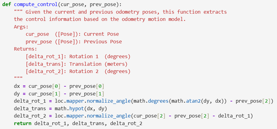
Extracts the rotation1, translation, and rotation2 control tuple from two consecutive odometry poses using math.hypot for translation and math.atan2 for heading, with angles normalized to [-180, 180) via loc.mapper.normalize_angle.
odom_motion_model
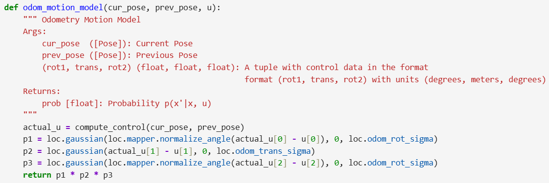
Computes the transition probability between a hypothetical previous and current pose. It calls compute_control to get the "required" control tuple, then compares each component against the actual odometry control tuple using a Gaussian. The three resulting probabilities (rotation1, translation, and rotation2) are multiplied together. Angles are explicitly normalized before evaluation to prevent wrap-around errors (e.g., incorrectly applying a massive penalty to the physical equivalence of 350° and -10°).
prediction_step
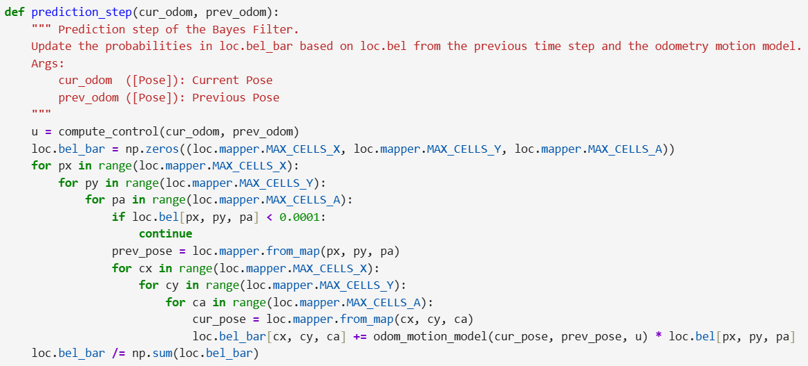
This step propagates the robot's belief state forward by iterating over all possible prior belief cells and applying the odometry motion model to distribute that probability into current cells. Because iterating over the full 3D grid against itself requires a massive number of loop executions, an aggressive optimization is implemented: any prior cell with a probability below 0.0001 is immediately skipped. For the remaining valid cells, loc.mapper.from_map is used to convert grid indices back into continuous physical poses before evaluating the motion model.
sensor_model
This function computes the likelihood of the 18 current ToF sensor readings given a specific hypothetical grid cell. Rather than using an explicit loop, it takes advantage of NumPy's optimized C-backend to perform a vectorized Gaussian evaluation. It compares the live sensor readings stored in loc.obs_range_data.flatten() against the precomputed ground truth distances for the given cell passed in as the obs array, using the predefined sensor standard deviation.

update_step
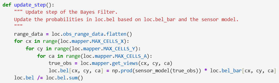
The update step incorporates the sensor data to refine the prior belief generated by the prediction step. For every cell in the grid, it fetches the ground truth sensor views using loc.mapper.get_views. It then calls sensor_model to get an array of 18 independent likelihoods, uses np.prod to combine them into a single probability scalar, and multiplies this by the cell's prior belief loc.bel_bar. Finally, to prevent arithmetic underflow and ensure a valid probability distribution, the entire 3D belief grid is divided by its sum to normalize the values back to 1.0.
Bayes Filter Results
The video below shows the Bayes filter running in the simulator across the full trajectory for Run 1. The green trajectory represents the ground truth path, the blue trajectory represents the odometry path, and the red trajectory represents the filter's most probable belief state at each timestep. As seen in the video, the belief closely tracks the ground truth throughout the run, demonstrating the filter's ability to correct for odometry drift using sensor updates.
Video showcasing the Bayes Filter.
The tables below show the most probable belief state after the update step at each timestep across three independent runs, compared against ground truth. Position values are in meters and angles are in degrees. While the ground truth state from the simulator accumulates angle without bounds, the belief state and the resulting angular error have been properly normalized to the [-180, 180) range to accurately reflect true heading deviation.
Run 1
| Step | Ground Truth State | Belief State | Belief Probability | Error | ||||||
|---|---|---|---|---|---|---|---|---|---|---|
| x (m) | y (m) | theta (deg) | x (m) | y (m) | theta (deg) | x (m) | y (m) | theta (deg) | ||
| 0 | 0.282 | -0.087 | 320.3 | 0.305 | 0.000 | -50.0 | 0.9999999 | -0.023 | -0.087 | 10.3 |
| 1 | 0.508 | -0.524 | 657.4 | 0.305 | -0.610 | -70.0 | 1.0 | 0.203 | 0.086 | 7.4 |
| 2 | 0.508 | -0.524 | 994.4 | 0.305 | -0.610 | -90.0 | 1.0 | 0.203 | 0.086 | 4.4 |
| 3 | 0.539 | -0.923 | 1354.4 | 0.610 | -0.914 | -90.0 | 1.0 | -0.071 | -0.008 | 4.4 |
| 4 | 0.799 | -1.062 | 1799.9 | 0.914 | -0.914 | 10.0 | 1.0 | -0.116 | -0.148 | -10.1 |
| 5 | 1.583 | -0.905 | 2208.9 | 1.524 | -0.914 | 50.0 | 1.0 | 0.059 | 0.010 | -1.1 |
| 6 | 1.668 | -0.521 | 2597.5 | 1.829 | -0.305 | 90.0 | 1.0 | -0.161 | -0.216 | -12.5 |
| 7 | 1.746 | -0.169 | 2963.2 | 1.829 | -0.305 | 90.0 | 1.0 | -0.083 | 0.136 | -6.8 |
| 8 | 1.756 | 0.322 | 3346.0 | 1.829 | 0.000 | 90.0 | 0.9999981 | -0.073 | 0.322 | 16.0 |
| 9 | 1.763 | 0.652 | 3745.1 | 1.829 | 0.914 | 150.0 | 1.0 | -0.066 | -0.262 | -4.9 |
| 10 | 1.353 | 0.938 | 4116.4 | 1.524 | 0.914 | 150.0 | 1.0 | -0.171 | 0.024 | 6.4 |
| 11 | 0.486 | 0.862 | 4573.8 | 0.610 | 0.914 | -110.0 | 1.0 | -0.124 | -0.053 | 3.8 |
| 12 | 0.305 | 0.237 | 4978.9 | 0.305 | 0.305 | -70.0 | 1.0 | -0.000 | -0.067 | 8.9 |
| 13 | 0.052 | -0.064 | 5270.1 | 0.000 | -0.305 | -130.0 | 1.0 | 0.052 | 0.240 | 0.1 |
| 14 | -0.319 | -0.214 | 5607.6 | -0.305 | -0.305 | -150.0 | 1.0 | -0.014 | 0.091 | -2.4 |
| 15 | -0.705 | -0.207 | 5944.6 | -0.610 | -0.305 | -170.0 | 0.9999999 | -0.096 | 0.098 | -5.4 |
Run 2
| Step | Ground Truth State | Belief State | Belief Probability | Error | ||||||
|---|---|---|---|---|---|---|---|---|---|---|
| x (m) | y (m) | theta (deg) | x (m) | y (m) | theta (deg) | x (m) | y (m) | theta (deg) | ||
| 0 | 0.282 | -0.086 | 320.6 | 0.305 | 0.000 | -50.0 | 0.9999999 | -0.023 | -0.086 | 10.6 |
| 1 | 0.510 | -0.521 | 657.6 | 0.305 | -0.610 | -70.0 | 1.0 | 0.206 | 0.088 | 7.6 |
| 2 | 0.510 | -0.521 | 994.7 | 0.305 | -0.610 | -90.0 | 1.0 | 0.206 | 0.088 | 4.7 |
| 3 | 0.543 | -0.920 | 1354.7 | 0.610 | -0.914 | -90.0 | 1.0 | -0.066 | -0.006 | 4.7 |
| 4 | 0.804 | -1.058 | 1800.2 | 0.914 | -0.914 | 10.0 | 1.0 | -0.111 | -0.144 | -9.8 |
| 5 | 1.581 | -0.898 | 2209.2 | 1.524 | -0.914 | 50.0 | 1.0 | 0.057 | 0.016 | -0.8 |
| 6 | 1.669 | -0.508 | 2597.3 | 1.829 | -0.305 | 90.0 | 1.0 | -0.160 | -0.203 | -12.7 |
| 7 | 1.747 | -0.157 | 2962.9 | 1.829 | -0.305 | 90.0 | 1.0 | -0.081 | 0.148 | -7.1 |
| 8 | 1.759 | 0.335 | 3345.5 | 1.829 | 0.000 | 90.0 | 0.9764887 | -0.069 | 0.335 | 15.5 |
| 9 | 1.769 | 0.659 | 3744.7 | 1.829 | 0.914 | 150.0 | 1.0 | -0.060 | -0.255 | -5.3 |
| 10 | 1.361 | 0.948 | 4115.9 | 1.524 | 0.914 | 150.0 | 1.0 | -0.163 | 0.034 | 5.9 |
| 11 | 0.463 | 0.884 | 4571.7 | 0.610 | 0.914 | -110.0 | 1.0 | -0.146 | -0.030 | 1.7 |
| 12 | 0.263 | 0.277 | 4977.5 | 0.305 | 0.305 | -70.0 | 1.0 | -0.042 | -0.027 | 7.5 |
| 13 | 0.009 | -0.024 | 5269.9 | 0.000 | 0.000 | -130.0 | 1.0 | 0.009 | -0.024 | -0.1 |
| 14 | -0.357 | -0.166 | 5606.9 | -0.305 | -0.305 | -150.0 | 1.0 | -0.052 | 0.138 | -3.1 |
| 15 | -0.750 | -0.155 | 5943.9 | -0.610 | -0.305 | -170.0 | 0.9996811 | -0.141 | 0.150 | -6.1 |
Run 3
| Step | Ground Truth State | Belief State | Belief Probability | Error | ||||||
|---|---|---|---|---|---|---|---|---|---|---|
| x (m) | y (m) | theta (deg) | x (m) | y (m) | theta (deg) | x (m) | y (m) | theta (deg) | ||
| 0 | 0.282 | -0.087 | 320.2 | 0.305 | 0.000 | -50.0 | 1.0 | -0.023 | -0.087 | 10.2 |
| 1 | 0.508 | -0.524 | 657.3 | 0.305 | -0.610 | -70.0 | 1.0 | 0.203 | 0.086 | 7.3 |
| 2 | 0.508 | -0.524 | 994.7 | 0.305 | -0.610 | -90.0 | 1.0 | 0.203 | 0.087 | 4.7 |
| 3 | 0.541 | -0.922 | 1354.8 | 0.610 | -0.914 | -90.0 | 1.0 | -0.068 | -0.008 | 4.8 |
| 4 | 0.802 | -1.060 | 1799.8 | 0.914 | -0.914 | 10.0 | 1.0 | -0.112 | -0.146 | -10.2 |
| 5 | 1.574 | -0.907 | 2209.1 | 1.524 | -0.914 | 50.0 | 1.0 | 0.050 | 0.008 | -0.9 |
| 6 | 1.660 | -0.523 | 2597.3 | 1.829 | -0.305 | 90.0 | 1.0 | -0.168 | -0.218 | -12.7 |
| 7 | 1.740 | -0.172 | 2962.9 | 1.829 | -0.305 | 90.0 | 0.9999999 | -0.089 | 0.133 | -7.1 |
| 8 | 1.751 | 0.320 | 3346.5 | 1.829 | 0.000 | 90.0 | 0.9981756 | -0.089 | 0.346 | 16.5 |
| 9 | 1.761 | 0.644 | 3745.9 | 1.829 | 0.914 | 150.0 | 1.0 | -0.086 | -0.239 | -4.1 |
| 10 | 1.353 | 0.933 | 4116.0 | 1.524 | 0.914 | 150.0 | 1.0 | -0.171 | 0.019 | 6.0 |
| 11 | 0.471 | 0.862 | 4572.2 | 0.610 | 0.914 | -110.0 | 1.0 | -0.139 | -0.052 | 2.2 |
| 12 | 0.272 | 0.243 | 4977.3 | 0.305 | 0.305 | -70.0 | 1.0 | -0.033 | -0.062 | 7.3 |
| 13 | 0.011 | -0.051 | 5268.5 | 0.000 | -0.305 | -130.0 | 0.9999999 | 0.011 | 0.253 | -1.5 |
| 14 | -0.358 | -0.185 | 5605.5 | -0.305 | -0.305 | -150.0 | 1.0 | -0.054 | 0.119 | -4.5 |
| 15 | -0.751 | -0.164 | 5942.6 | -0.610 | -0.305 | -170.0 | 0.8739048 | -0.142 | 0.141 | -7.4 |
Overall the filter performs well across all three runs using the default sample trajectory, with x and y position errors consistently staying within one grid cell width (0.3048 m). The angular errors after normalization are small throughout, generally staying within roughly 10-17 degrees, which is less than one grid cell in the theta dimension (20 degrees). Results are consistent across all three runs, with the filter converging to the same solution each time.
The update step is clearly the dominant source of accuracy. While the prediction step alone would produce a diffuse belief spread across multiple cells due to noisy odometry, the 18-reading sensor update provides enough information to sharply localize the robot, converging probabilities near 1.0. The filter struggles slightly before initial convergence, and at timestep 15 in run 3 the probability dips to 0.874, likely due to accumulated odometry drift and a noisier sensor sweep. Despite this, the positional estimate remains within one grid cell of ground truth.
Aidan McNay's website was used to inspire sections of this lab.